38
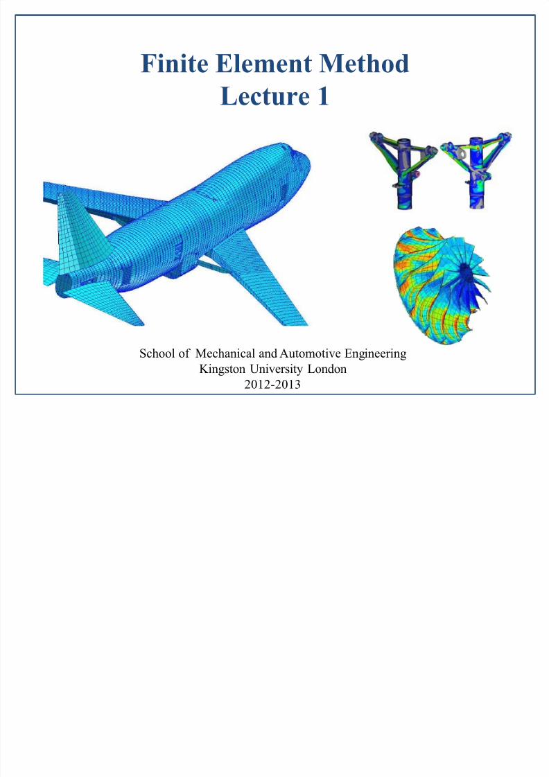
Finite Element Method Lecture 1 School of Mechanical and Automotive Engineering Kingston University London 2012-2013
| Date post: | 03-Apr-2018 |
| Category: |
Documents |
| Upload: | sabine-brosch |
| View: | 226 times |
| Download: | 0 times |
7/28/2019 Lectuer 1- Sami Vahid-1
http://slidepdf.com/reader/full/lectuer-1-sami-vahid-1 1/38
Finite Element Method
Lecture 1
School of Mechanical and Automotive Engineering
Kingston University London
2012-2013

7/28/2019 Lectuer 1- Sami Vahid-1
http://slidepdf.com/reader/full/lectuer-1-sami-vahid-1 2/38
Lecture 1: Finite Element Method

7/28/2019 Lectuer 1- Sami Vahid-1
http://slidepdf.com/reader/full/lectuer-1-sami-vahid-1 3/38
Design analysis: hand calculations, experiments, and
computer simulations
FEA is the most widely applied computer simulation
method in engineering
Closely integrated with CAD/CAM applications
Why Finite Element Method?

7/28/2019 Lectuer 1- Sami Vahid-1
http://slidepdf.com/reader/full/lectuer-1-sami-vahid-1 4/38
Applications of FEM in
Engineering
• Mechanical/Aerospace/Civil/Automobile Engineering
• Structure analysis (static/dynamic, linear/nonlinear)
• Thermal/fluid flows
• Electromagnetics
• Geomechanics
•
Biomechanics• …..
7/28/2019 Lectuer 1- Sami Vahid-1
http://slidepdf.com/reader/full/lectuer-1-sami-vahid-1 5/38
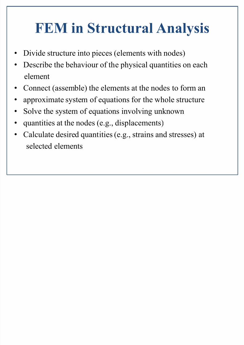
FEM in Structural Analysis
• Divide structure into pieces (elements with nodes)
• Describe the behaviour of the physical quantities on each
element
• Connect (assemble) the elements at the nodes to form an
• approximate system of equations for the whole structure
• Solve the system of equations involving unknown
• quantities at the nodes (e.g., displacements)
• Calculate desired quantities (e.g., strains and stresses) at
selected elements

7/28/2019 Lectuer 1- Sami Vahid-1
http://slidepdf.com/reader/full/lectuer-1-sami-vahid-1 6/38
Example

7/28/2019 Lectuer 1- Sami Vahid-1
http://slidepdf.com/reader/full/lectuer-1-sami-vahid-1 7/38
Computer Implementations
• Preprocessing (build FE model, loads and constraints)
• FEA solver (assemble and solve the system of equations)
• Postprocessing (sort and display the results)
7/28/2019 Lectuer 1- Sami Vahid-1
http://slidepdf.com/reader/full/lectuer-1-sami-vahid-1 8/38
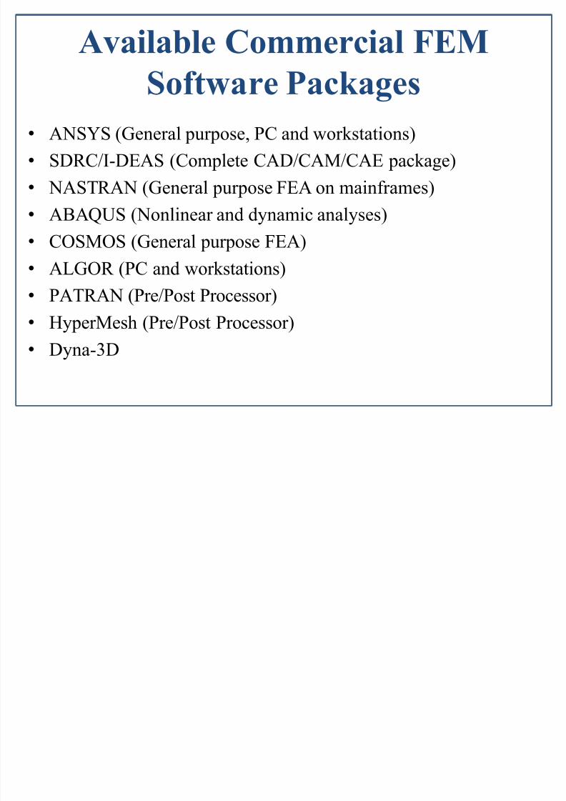
• ANSYS (General purpose, PC and workstations)
• SDRC/I-DEAS (Complete CAD/CAM/CAE package)
• NASTRAN (General purpose FEA on mainframes)
• ABAQUS (Nonlinear and dynamic analyses)
• COSMOS (General purpose FEA)
• ALGOR (PC and workstations)
• PATRAN (Pre/Post Processor)• HyperMesh (Pre/Post Processor)
• Dyna-3D
Available Commercial FEM
Software Packages

7/28/2019 Lectuer 1- Sami Vahid-1
http://slidepdf.com/reader/full/lectuer-1-sami-vahid-1 9/38
Structural analysis is based on the following four principles:
(1) Equilibrium of forces
(2) Constitutive equations (material properties)
(3) Compatibility of displacements(4) Boundary conditions
Application of (1) – (3) will lead in general to a second order
partial differential equation that can be solved using finite
elements or other techniques by applying (4).
Structural Background

7/28/2019 Lectuer 1- Sami Vahid-1
http://slidepdf.com/reader/full/lectuer-1-sami-vahid-1 10/38
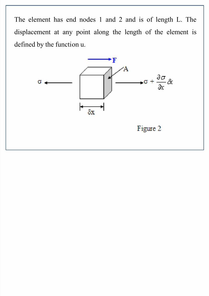
Example:
Consider the equilibrium of a uniform beam under the action of
axial forces, see Figure 1
7/28/2019 Lectuer 1- Sami Vahid-1
http://slidepdf.com/reader/full/lectuer-1-sami-vahid-1 11/38
The element has end nodes 1 and 2 and is of length L. The
displacement at any point along the length of the element is
defined by the function u.

7/28/2019 Lectuer 1- Sami Vahid-1
http://slidepdf.com/reader/full/lectuer-1-sami-vahid-1 12/38
Over a small length x of the element (see Figure 2), the variation
of stress will be given by
x x
Hence, the resultant internal force in the x-direction will be given
by A x
x
.
If the element is subjected to an external force F per unit length,
then for equilibrium0
x
x A F
0
F
x A

7/28/2019 Lectuer 1- Sami Vahid-1
http://slidepdf.com/reader/full/lectuer-1-sami-vahid-1 13/38
But, (constitutive equation).
Over a small length, the longitudinal strain is defined as the rate
of change of longitudinal displacement i.e.
Hence the equilibrium equation becomes
E
0 F x
AE
x
u
.02
2
F
x
u AE

7/28/2019 Lectuer 1- Sami Vahid-1
http://slidepdf.com/reader/full/lectuer-1-sami-vahid-1 14/38
The equilibrium equation is thus a second order partial
differential equation which can be solved by the finite element
method once the appropriate boundary conditions e.g.
displacements at nodes 1 and 2 are known.
7/28/2019 Lectuer 1- Sami Vahid-1
http://slidepdf.com/reader/full/lectuer-1-sami-vahid-1 15/38
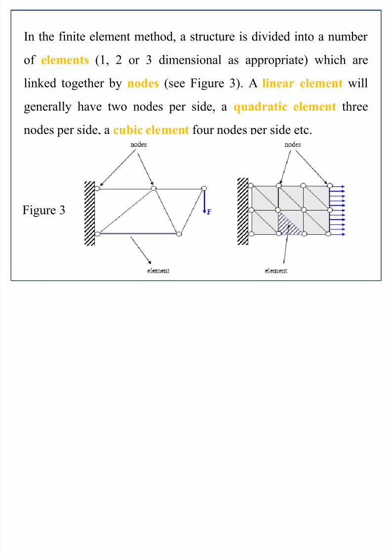
In the finite element method, a structure is divided into a number
of elements (1, 2 or 3 dimensional as appropriate) which are
linked together by nodes (see Figure 3). A linear element will
generally have two nodes per side, a quadratic element three
nodes per side, a cubic element four nodes per side etc.
Figure 3

7/28/2019 Lectuer 1- Sami Vahid-1
http://slidepdf.com/reader/full/lectuer-1-sami-vahid-1 16/38
Application of the finite element method results in a loaded
structure being represented by the matrix equation
where F is a vector of the external nodal applied load, is a
vector of the nodal displacements and K is the overall (global)stiffness matrix which is formed from an assemblage of the
individual element stiffness matrices K e.
F = K
7/28/2019 Lectuer 1- Sami Vahid-1
http://slidepdf.com/reader/full/lectuer-1-sami-vahid-1 17/38
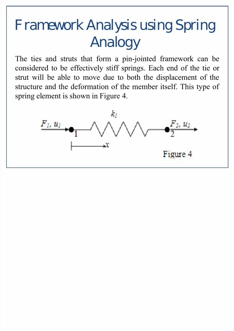
The ties and struts that form a pin-jointed framework can be
considered to be effectively stiff springs. Each end of the tie or
strut will be able to move due to both the displacement of the
structure and the deformation of the member itself. This type of
spring element is shown in Figure 4.
Framework Analysis using Spring
Analogy

7/28/2019 Lectuer 1- Sami Vahid-1
http://slidepdf.com/reader/full/lectuer-1-sami-vahid-1 18/38
The element has two nodes 1 and 2. The displacement and applied
force at node 1 are u1 and F1 and the displacement and applied
force at node 2 are u2 and F2. The element has length L and cross-
sectional area A.
The stiffness of the element will be given by where E isYoung’s modulus.
If externally applied forces F1 and F2 induce displacements u1 and
u2 at nodes 1 and 2 respectively then
L
AE
k
1
21112111
uk uk uuk F
21111212
uk uk uuk F
7/28/2019 Lectuer 1- Sami Vahid-1
http://slidepdf.com/reader/full/lectuer-1-sami-vahid-1 19/38
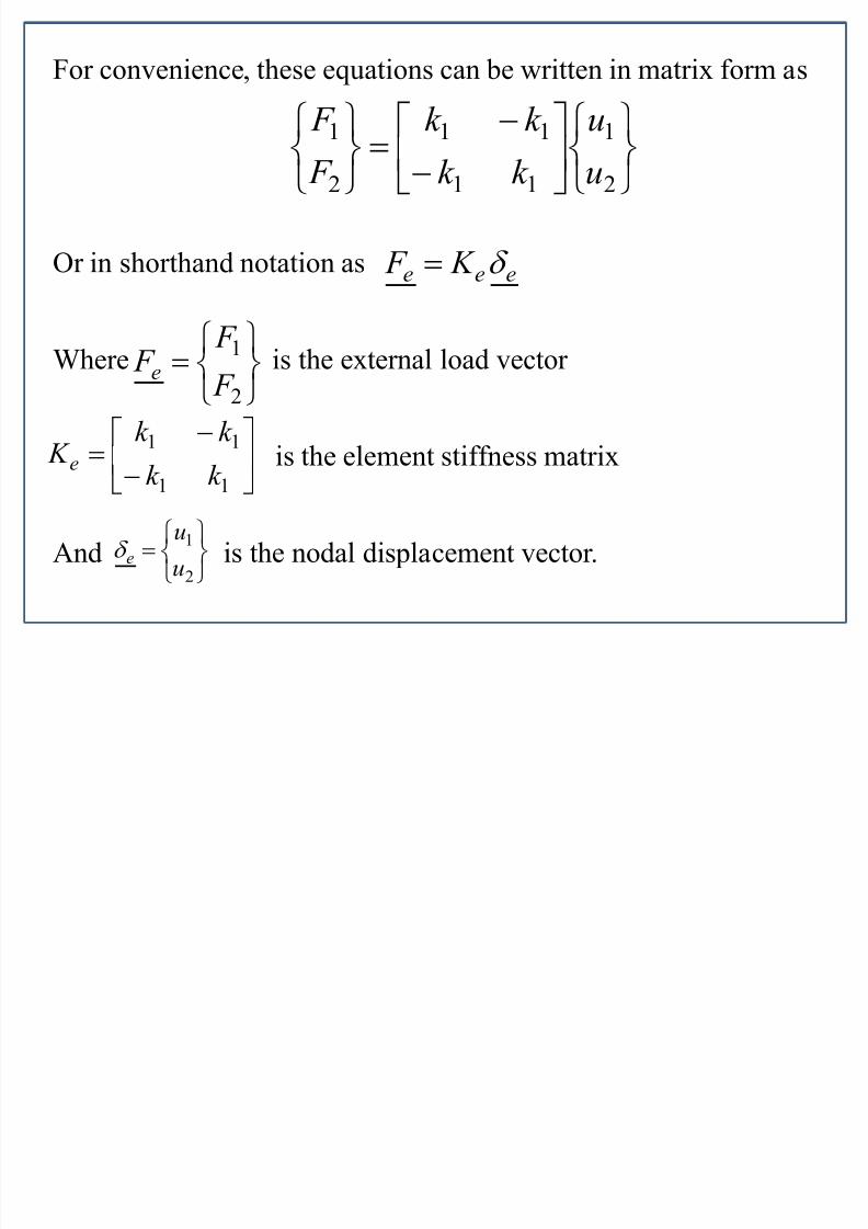
For convenience, these equations can be written in matrix form as
Or in shorthand notation as
Where is the external load vector
is the element stiffness matrix
And is the nodal displacement vector.
2
1
11
11
2
1
u
u
k k
k k
F
F
eee K F
2
1
F
F F e
11
11
k k
k k
K e
2
1
u
ue
7/28/2019 Lectuer 1- Sami Vahid-1
http://slidepdf.com/reader/full/lectuer-1-sami-vahid-1 20/38
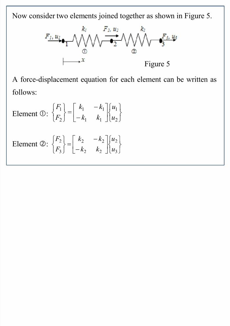
Now consider two elements joined together as shown in Figure 5.
A force-displacement equation for each element can be written asfollows:
Element:
Element:
2
1
11
11
2
1
u
u
k k
k k
F
F
3
2
22
22
3
2
u
u
k k
k k
F
F
Figure 5

7/28/2019 Lectuer 1- Sami Vahid-1
http://slidepdf.com/reader/full/lectuer-1-sami-vahid-1 21/38
Expanding both matrices so that they are in an equivalent form
gives:
and
The overall force-displacement matrix can be obtained by adding
these two matrices together. Thus:
3
2
1
22
22
3
2
1
0
0
000
u
u
u
k k
k k
F
F
F
3
2
1
11
11
3
2
1
000
0
0
u
u
u
k k
k k
F
F
F
3
2
1
22
2211
11
3
2
1
0
0
u
u
u
k k
k k k k
k k
F
F
F

7/28/2019 Lectuer 1- Sami Vahid-1
http://slidepdf.com/reader/full/lectuer-1-sami-vahid-1 22/38
Or
where FG is the global force vector, K G is the global stiffness
matrix and G is the global displacement vector.
GGG K F

7/28/2019 Lectuer 1- Sami Vahid-1
http://slidepdf.com/reader/full/lectuer-1-sami-vahid-1 23/38
Example 1:
Three dissimilar materials are friction welded together and
mounted between rigid end supports as shown in Figure Q1.If forces of 100 kN and 50 kN are applied as indicated, find the
movement of the interfaces between the materials and the forces
on the end supports. Material properties are given in Table Q1.
Aluminium Brass Steel
Area (mm2) 400 200 70
Length (mm) 280 100 100
E (GPa) 70 100 200
Table Q1
Figure Q1

7/28/2019 Lectuer 1- Sami Vahid-1
http://slidepdf.com/reader/full/lectuer-1-sami-vahid-1 24/38
Solution
Spring stiffness will be k 1 = 100 kN/mm, k 2 = 200 kN/mm and
k 3 = 140 kN/mm.
7/28/2019 Lectuer 1- Sami Vahid-1
http://slidepdf.com/reader/full/lectuer-1-sami-vahid-1 25/38
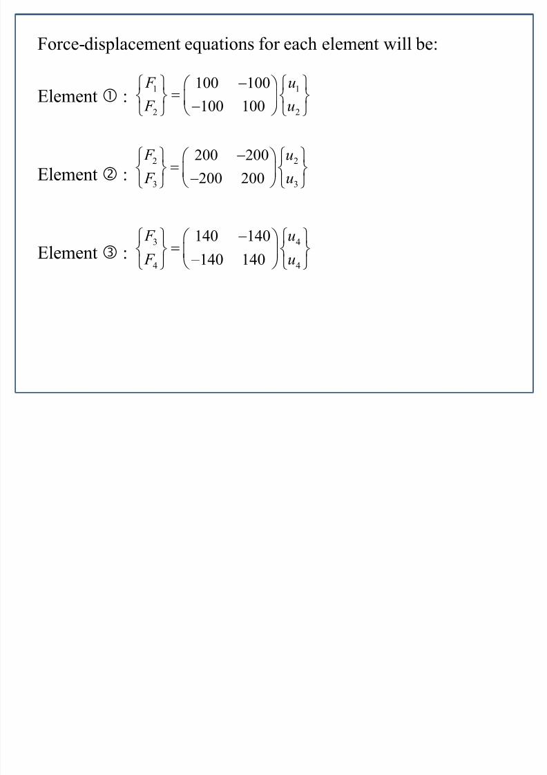
Force-displacement equations for each element will be:
Element :
Element :
Element :
1 1
2 2
100 100
100 100
F u
F u
2 2
3 3
200 200
200 200
F u
F u
3 4
4 4
140 140
140 140
F u
F u
7/28/2019 Lectuer 1- Sami Vahid-1
http://slidepdf.com/reader/full/lectuer-1-sami-vahid-1 26/38
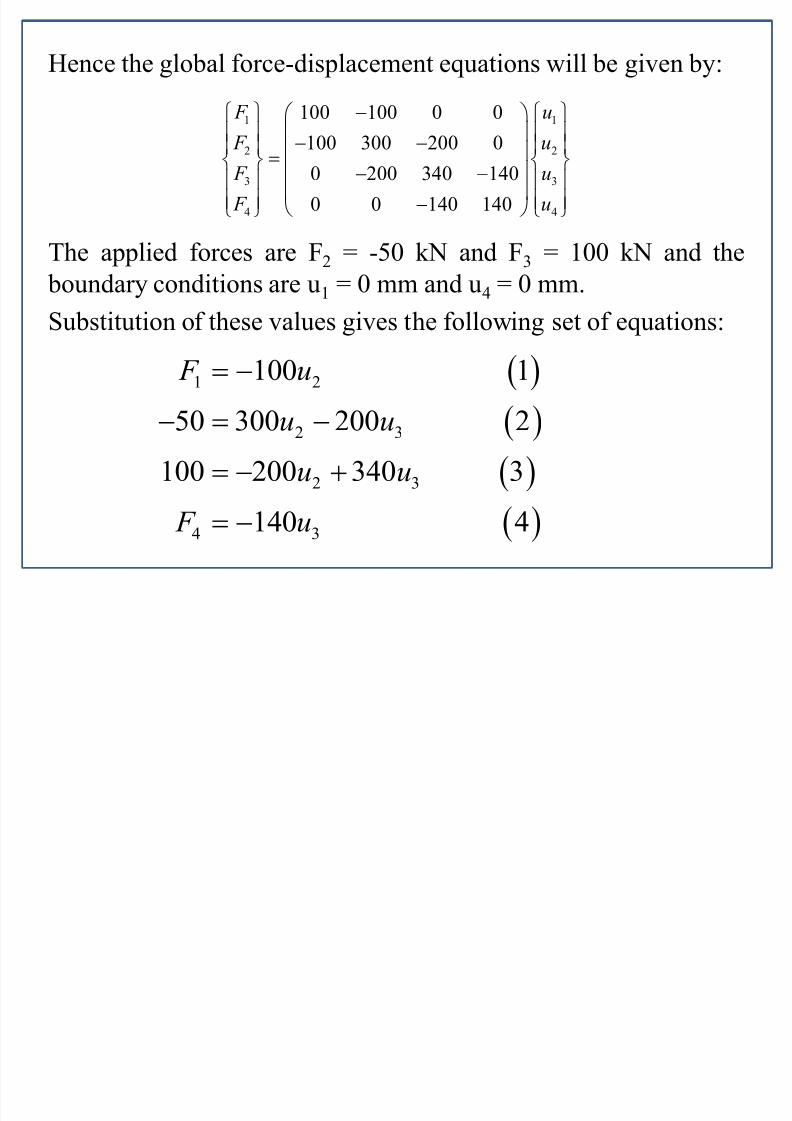
Hence the global force-displacement equations will be given by:
The applied forces are F2 = -50 kN and F3 = 100 kN and the
boundary conditions are u1 = 0 mm and u4 = 0 mm.
Substitution of these values gives the following set of equations:
1 1
2 2
3 3
4 4
100 100 0 0
100 300 200 0
0 200 340 140
0 0 140 140
F u
F u
F u
F u
1 2
2 3
2 3
4 3
100 1
50 300 200 2
100 200 340 3
140 4
F u
u u
u u
F u

7/28/2019 Lectuer 1- Sami Vahid-1
http://slidepdf.com/reader/full/lectuer-1-sami-vahid-1 27/38
Solving equations (2) and (3) gives u2 = 0.048 mm and u3 = 0.323
mm.
Substitution in equations (1) and (4) gives F1 = -4.8 kN andF4 = -45.2 kN.
7/28/2019 Lectuer 1- Sami Vahid-1
http://slidepdf.com/reader/full/lectuer-1-sami-vahid-1 28/38
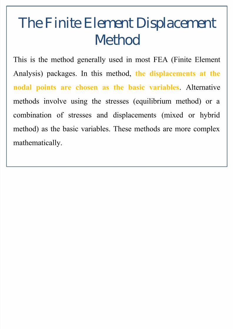
This is the method generally used in most FEA (Finite Element
Analysis) packages. In this method, the displacements at the
nodal points are chosen as the basic variables. Alternative
methods involve using the stresses (equilibrium method) or a
combination of stresses and displacements (mixed or hybrid
method) as the basic variables. These methods are more complex
mathematically.
The Finite Element Displacement
Method
7/28/2019 Lectuer 1- Sami Vahid-1
http://slidepdf.com/reader/full/lectuer-1-sami-vahid-1 29/38
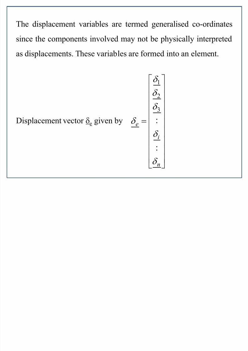
The displacement variables are termed generalised co-ordinates
since the components involved may not be physically interpreted
as displacements. These variables are formed into an element.
Displacement vector e given by
n
i
e
:
:
3
2
1
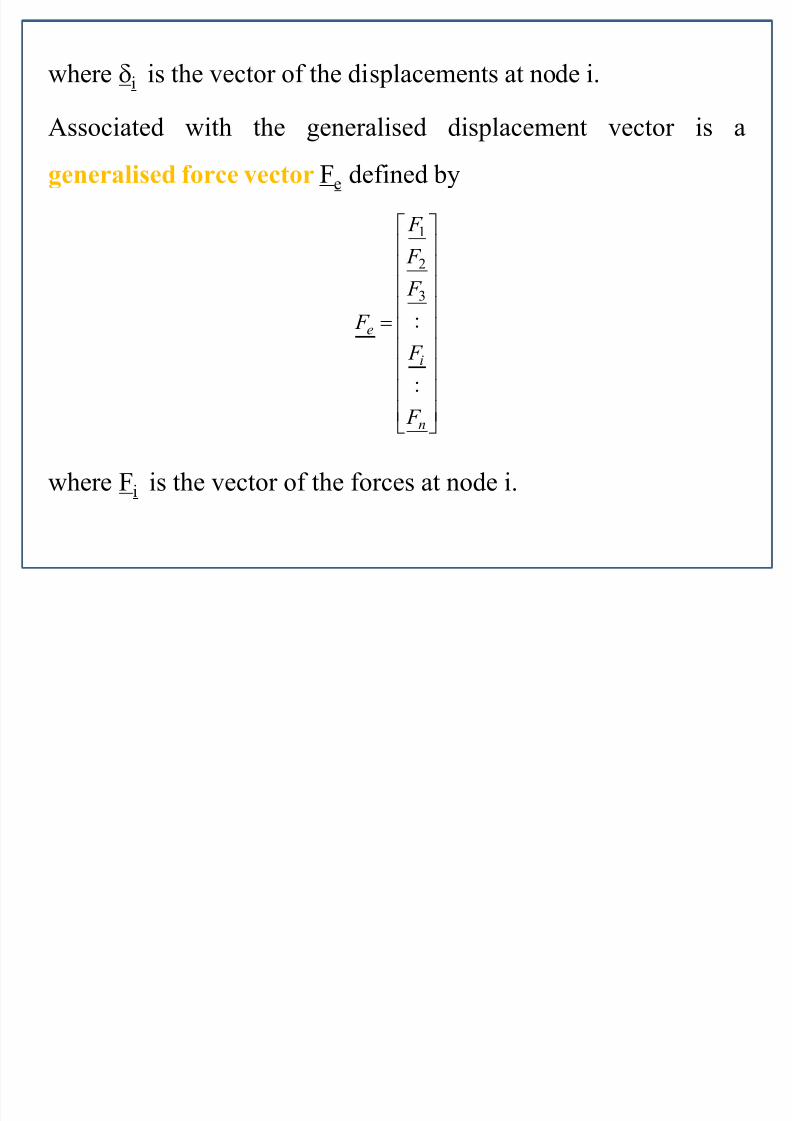
7/28/2019 Lectuer 1- Sami Vahid-1
http://slidepdf.com/reader/full/lectuer-1-sami-vahid-1 30/38
where i is the vector of the displacements at node i.
Associated with the generalised displacement vector is a
generalised force vector Fe defined by
where Fi is the vector of the forces at node i.
n
i
e
F
F
F
F
F
F
:
:
3
2
1
7/28/2019 Lectuer 1- Sami Vahid-1
http://slidepdf.com/reader/full/lectuer-1-sami-vahid-1 31/38
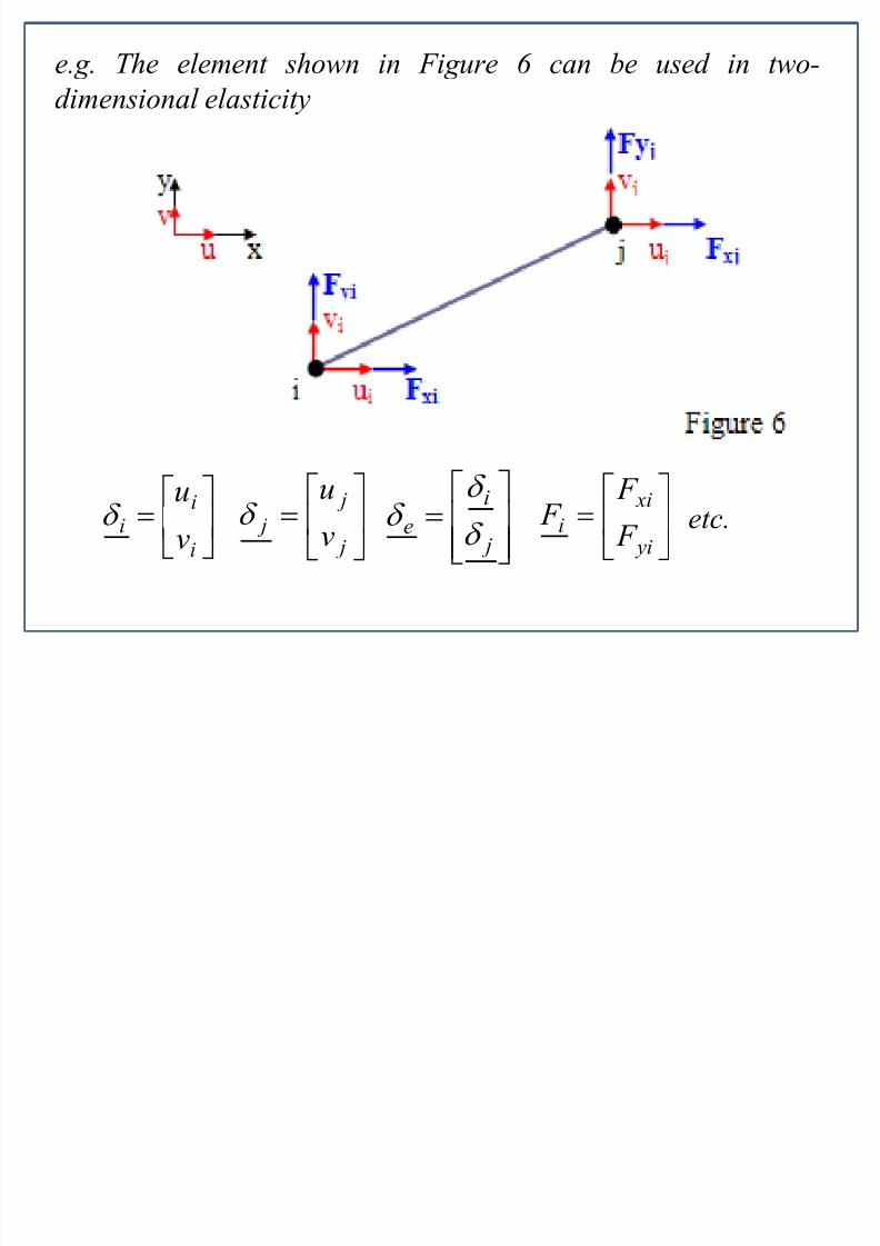
e.g. The element shown in Figure 6 can be used in two-
dimensional elasticity
etc.
i
ii
v
u
j
j
j v
u
j
i
e
yi
xi
i F
F F

7/28/2019 Lectuer 1- Sami Vahid-1
http://slidepdf.com/reader/full/lectuer-1-sami-vahid-1 32/38
e.g. The element shown in Figure 7 can be used in plate bendingtheory
In stress analysis, the product of the generalised forces and thegeneralised displacements must give work.
yi
xi
i
i
w
p
j
i
e
.
yi
xi
i
i
M
M
F
F
p
j
i
e
F
F
F
F .

7/28/2019 Lectuer 1- Sami Vahid-1
http://slidepdf.com/reader/full/lectuer-1-sami-vahid-1 33/38
Shape functions are used to define the assumed variation of a
particular variable e.g. displacement over the whole domain of an
element.
Shape Functions

7/28/2019 Lectuer 1- Sami Vahid-1
http://slidepdf.com/reader/full/lectuer-1-sami-vahid-1 34/38
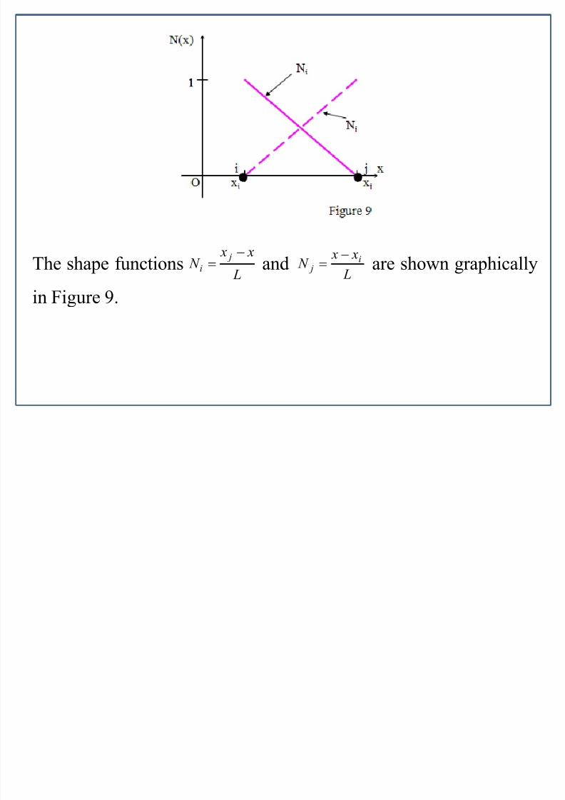
The element shown in Figure 8, which lies along the x-axis, has
two nodes i and j with co-ordinates xi and x j respectively. A
quantity is assumed to vary linearly across the element and has
values i and j at nodes i and j.
Since is assumed to vary linearly, it will be represented by theequation where a1 and a2 are constants.
and
Since = i at x = xi, and = j at x = x j, then
L
x x
x x
x xa
i j ji
i j
i j ji
1 L x xa
i j
i j
i j
2

7/28/2019 Lectuer 1- Sami Vahid-1
http://slidepdf.com/reader/full/lectuer-1-sami-vahid-1 35/38
Hence
In matrix form = N where N = and
The functions and are the shape functions
and show the variation of i and j respectively over the domain
of the element.
j jii ji
i
ji ji j ji N N
L
x x
L
x x x
L L
x x
ji N N
j
i
L
x x N
j
i
L
x x
N i
j

7/28/2019 Lectuer 1- Sami Vahid-1
http://slidepdf.com/reader/full/lectuer-1-sami-vahid-1 36/38
Example 2: The nodal co-ordinates xi and x j of an element are
3.0 cm and 4.5 cm respectively. The temperatures at these nodes
are found to be 27°C and 33°C respectively. What is the
temperature at x = 3.6 cm?
and
Hence at x = 3.6 cm,
4.5
1.5
j
i
x x x
N L
3.0
1.5 j
x N
4.5 3.6 3.6 3.027 33
1.5 1.5
0.6 27 0.4 33
29.4
T
C
7/28/2019 Lectuer 1- Sami Vahid-1
http://slidepdf.com/reader/full/lectuer-1-sami-vahid-1 37/38
The shape functions and are shown graphically
in Figure 9.
L
x x N
j
i
L
x x N i
j
7/28/2019 Lectuer 1- Sami Vahid-1
http://slidepdf.com/reader/full/lectuer-1-sami-vahid-1 38/38
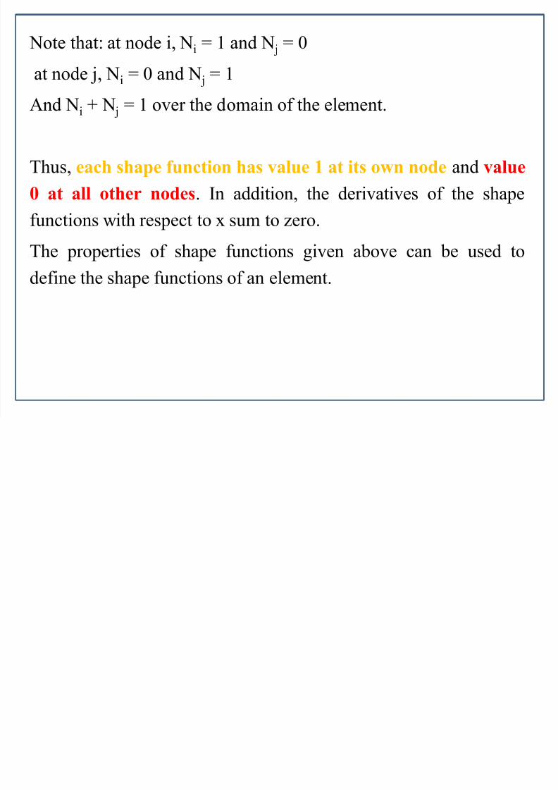
Note that: at node i, Ni = 1 and N j = 0
at node j, Ni = 0 and N j = 1
And Ni + N j = 1 over the domain of the element.
Thus, each shape function has value 1 at its own node and value
0 at all other nodes. In addition, the derivatives of the shapefunctions with respect to x sum to zero.
The properties of shape functions given above can be used to
define the shape functions of an element.


