216
Visual SLAM, Bundle Adjustment, Factor Graphs Frank Dellaert, Robotics & Intelligent Machines @ Georgia Tech

Visual SLAM, Bundle Adjustment, Factor Graphs Frank Dellaert, Robotics & Intelligent Machines @ Georgia Tech

Intro Visual SLAM
Bundle Adjustment Factor Graphs Incremental Large-‐Scale
End
Outline
2
Intro Visual SLAM
Bundle Adjustment Factor Graphs Incremental Large-‐Scale
End

Frank Dellaert: Optimization in Factor Graphs for Fast and Scalable 3D Reconstruction and Mapping 3
2014

Frank Dellaert
Monte Carlo Localization
Dellaert, Fox, Burgard & Thrun, ICRA 1999

Frank Dellaert
Monte Carlo Localization
Dellaert, Fox, Burgard & Thrun, ICRA 1999

Frank Dellaert: Inference in Factor Graphs, Tutorial at ICRA 2013
Biotracking
• Multi-Target Tracking with MCMC
5

Frank Dellaert: Inference in Factor Graphs, Tutorial at ICRA 2013
Biotracking
• Multi-Target Tracking with MCMC
5

Frank Dellaert: Inference in Factor Graphs, Tutorial at ICRA 2013 6
SFM without Correspondence

Frank Dellaert
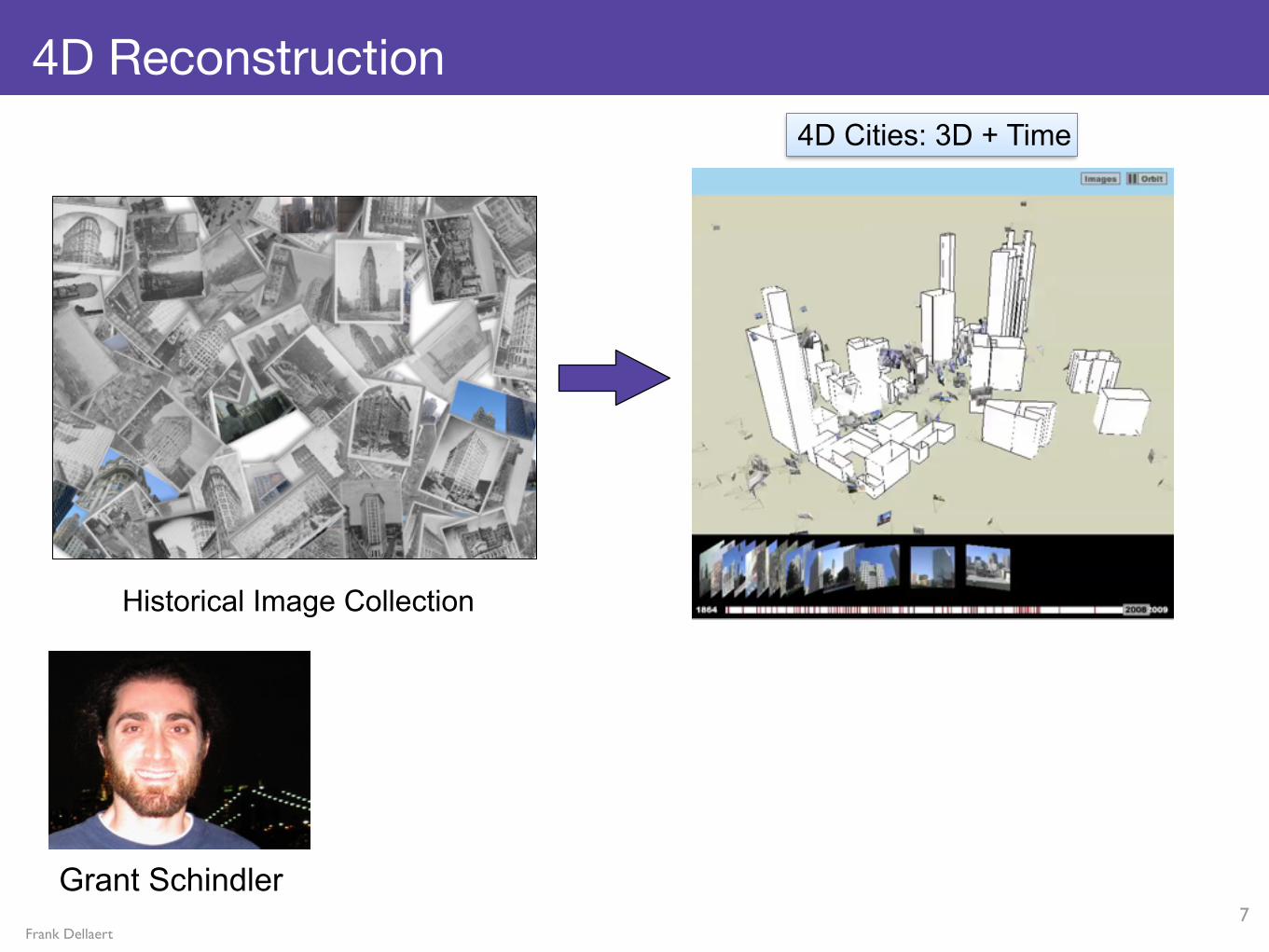
4D Reconstruction
7
Historical Image Collection
4D City Model
4D Cities: 3D + Time
Grant Schindler
Frank Dellaert
4D Reconstruction
7
Historical Image Collection
4D City Model
4D Cities: 3D + Time
Grant Schindler

Frank Dellaert
4D Reconstruction
7
Historical Image Collection
4D City Model
4D Cities: 3D + Time
Grant Schindler

Frank Dellaert: Inference in Factor Graphs, Tutorial at ICRA 2013
4D Structure over Time
8

Frank Dellaert: Inference in Factor Graphs, Tutorial at ICRA 2013
4D Structure over Time
8

Frank Dellaert: Optimization in Factor Graphs for Fast and Scalable 3D Reconstruction and Mapping
Large-Scale Structure from Motion
Photo Tourism
[Snavely et al. SIGGRAPH’06]
Build Rome in a Day
[Agarwal et al. ICCV’09]
Photosynth
[Microsoft]
Build Rome on a Cloudless Day
[Frahm et al. ECCV’10]
Iconic Scene Graphs
[Li et al. ECCV’08]
Discrete-Continuous Optim.
[Crandall et al. CVPR’11]
2 / 40���9Frank Dellaert: Optimization in Factor Graphs for Fast and Scalable 3D Reconstruction and Mapping

Frank Dellaert: Optimization in Factor Graphs for Fast and Scalable 3D Reconstruction and Mapping
3D Models from Community Databases
• E.g., Google image search on “Dubrovnik”
10

Frank Dellaert: Optimization in Factor Graphs for Fast and Scalable 3D Reconstruction and Mapping
3D Models from Community Databases
Agarwal, Snavely et al., University of Washingtonhttp://grail.cs.washington.edu/rome/
115K images, 3.5M points, >10M factors

Frank Dellaert: Optimization in Factor Graphs for Fast and Scalable 3D Reconstruction and Mapping
3D Models from Community Databases
Agarwal, Snavely et al., University of Washingtonhttp://grail.cs.washington.edu/rome/
115K images, 3.5M points, >10M factors

Intro Visual SLAM
Bundle Adjustment Factor Graphs Incremental Large-‐Scale
End
Outline
12
Intro Visual SLAM
Bundle Adjustment Factor Graphs Incremental Large-‐Scale
End

Bibliography• Murray, Li & Sastry, 1994 • Hartley and Zisserman, 2004 • Visual Odometry, Nister et al, CVPR 2004 • An Invitation to 3-‐D Vision, Ma, Soatto, Kosecka, Sastry, 2005 • Square Root SAM, Dellaert & Kaess, IJRR 2006 • Absil, Mahony & Sepulchre, 2007 • iSAM, Kaess & Dellaert, TRO 2008 • iSAM 2, Kaess et al, IJRR 2011 • Generalized Subgraph Preconditioners, Jian et al, ICCV 2011 • Visibility Based Preconditioning, Kushal & Agarwal, CVPR 2012 • CVPR 2014 Tutorial on Visual SLAM,
http://frc.ri.cmu.edu/~kaess/vslam_cvpr14/

Intro Visual SLAM
Bundle Adjustment Factor Graphs Incremental Large-‐Scale
End
Outline
14
Intro Visual SLAM
Bundle Adjustment Factor Graphs Incremental Large-‐Scale
End

What is Visual Odometry?

What is Visual Odometry?

What is Visual Odometry?

Monocular Visual Odometry
16
• VO: two frames -‐> R,t • Essential Matrix • 5-‐point RANSAC algorithm • Refinement

• Why Stereo? • Avoids scale ambiguity inherent in monocular VO • No special initialization procedure of landmark depth
Stereo Visual Odometry

Stereo VO Overview1. Rectification
2. Feature Extraction
4. Temporal Feature Matching
3. Stereo Feature Matching
5. Incremental Pose Recovery/RANSAC

Undistortion and Rectification

• Detect local features in each image • SIFT gives good results (can also use SURF, Harris, etc.)
Feature Extraction
Lowe ICCV 1999

• Match features between left/right images
• Since the images are rectified, we can restrict the search to a bounding box on the same scan-line
Stereo Matching
Left image Right image

• Temporally match features between frame t and t-1
Temporal Matching

• There will be some erroneous stereo and temporal feature associations à Use 3-point RANSAC
• Select 3 correspondences at random • Estimate relative transform R,t • Find the fraction of inliers that agree with this transform • Repeat for fixed nr. of tries or until fraction>80%
• Compute refined model using full inlier set
Relative Pose Estimation/RANSAC

• Camera pose can be recovered given at least three known landmarks in a non-degenerate configuration
• In the case of stereo VO, landmarks can simply be triangulated
• Two ways to recover pose: • Absolute orientation • Reprojection error minimization
Relative Pose Estimation
6 DOF camera pose
Known 3D landmarks

• Estimate relative relative transformation between 3D landmarks which were triangulated from stereo-matched features
• 3-Point algorithm: polynomial equations
Absolute Orientation
Pose r0
Pose r1Tt
Pose r0
(R,t) ? Tt-1
Tt-1
Tt

• Another approach is to estimate relative pose by minimizing reprojection error of 3D landmarks into images at time t and t-1
• Even better: jointly optimize the landmark positions and the relative camera pose:
• the measurement function h(.) transforms 3D points into the camera frame at time t, and then projects into the stereo images
Relative Pose Estimation
26
Camera posesLandmarksMeasurements
technique produces similar results whether we use SIFT orSURF, with SURF running significantly faster. The resultsin this paper were generated using only SURF features.
Given the SURF features, we establish matches betweenleft and right images in the usual manner. Specifically, weextract SURF features in both images of a stereo pair,which both generate a 128-element feature descriptor. Wethen establish stereo matches by computing the Euclideandistance between feature descriptors found in the left andright images. The images are rectified, and as a consequencewe are able to restrict the search for stereo correspondencesto the epipolar line, and a small region above/below becausethe calibration may not be perfect. We are mostly interestedin tracking features which are within a few meters of thestereo rig, allowing us to further restrict our search windowto a certain range of disparities. Restricting the search inthis fashion minimizes the computational time expended onstereo matching. The 3D coordinate of each point for whicha stereo match was found is computed using the reprojectionmatrix Q introduced in section III, and stored for lateruse. The resulting 3D points represent the initial positionestimates of the landmarks/vertices in a single frame.
B. Temporal Matching and RANSAC
We track features from frame to frame to recover thestructure of the environment. At each iteration, features arematched temporally by individually comparing each featuredescriptor from the current pair of images to the featuredescriptors in the previous pair of images, restricted to asmall search region within the previous image. A linearmotion model in image space is used to estimate the positionof potential matches. This speeds up the search, and addi-tionally reduces the number of erroneous matches. Putativesare established by computing the Euclidean distance betweenthe 128-element feature descriptors, similar to what was donepreviously for establishing stereo correspondences.
The incremental rotation R and translation t which expressthe current frame’s camera pose with respect to the previousone are recovered by way of applying a three point algorithmwithin a RANSAC framework. SIFT and SURF descriptormatching are quite reliable in many situations, yet RANSACis needed to eliminate outliers due to erroneous stereo andtemporal matching, as outliers are capable of introducinglarge error into the solution. Composing the incrementalrotation and translation for each new stereo rig pose withthe previous stereo rig pose yields a camera trajectory in theglobal coordinate frame. Putative inliers are saved to be usedfor batch smoothing and mapping in the following stage.
V. 3D POINT CLOUD AND CAMERA TRAJECTORYOPTIMIZATION
A. Smoothing and Mapping
Smoothing and Mapping (SAM) is a smoothing (insteadof filtering) approach to the SLAM estimation problem [4],[17]. It is a powerful tool based on graphical models whichhas been efficiently used to estimate the location of a set
Fig. 1. Factor Graph of two camera poses r and three landmarks l
of landmarks in the environment together with the cameratrajectory.
SAM enables large-scale mapping, is highly accurate, yetremains efficient in contrast to the state of the art methodsbased on filtering. While these methods work by estimatingonly the current state of the vehicle, SAM solves for theentire vehicle trajectory (smoothing), i.e. the position of theunderwater vehicle throughout the entire mission. Paradox-ically, it was shown in [4], [17] that by asking for more(full trajectories) the resulting optimization problems remainsparse which results in more efficient mapping algorithmsthan in the filtering paradigm. In addition, the smoothingapproach does not suffer from the consistency issues thatare typical in filtering methods: because the full trajectoryis always there to re-linearize around, smoothing providesa gold-standard 3D reconstruction that cannot be achievedby any extended Kalman filter approach that ”solidifies”linearization errors into the solution.
Factor graphs offer a straightforward and natural way tothink of the SAM problem. Fig. 1 shows an illustration ofa factor graph which is representative of the optimizationproblem. The factor graph fully represents the problem to besolved in a graphical way, where the 6 DOF poses of the leftstereo rig camera are indicated by r, and the tracked SURFlandmarks are denoted as l, where landmarks are representedas 3D points. The nodes on the vertices connecting thevariables r and l represent the visual image measurementsthat were made for each tracked feature point.
We optimize over the entire set of camera poses andlandmarks, R and L respectively, and collect all unknownsin the vector ⇥
�= (R,L). The factor graph then captures a
non-linear least-squares problem
⇥⇤ �= argmin
⇥
MX
m=1
khm
(rim , l
jm)� zm
k2⌃m(4)
where h
m
(·) is the measurement function of landmark l
jm
from pose r
im , and M is the total number of measurements,and r 2 R and l 2 L .The measurements are denoted byzm
= (uL
, u
R
, v), where u
L
and u
R
are the horizontalpixel coordinates, and v the vertical pixel coordinate, all ofwhich result from the projection of a tracked 3D point intothe stereo pair. Only one value is needed for v because the
Triangulate
Tt
Tt-1
Reproject
Tt
Tt-1

• The presented algorithm works very well in feature-rich, static environments, but…
• A few tricks for better results in challenging conditions: • Feature binning to cope with bias due to uneven feature
distributions • Keyframing to cope with dynamic scenes, as well as reducing
drift of a stationary camera
• Real-time performance
Practical/Robustness Considerations

• Incremental pose estimation yields poor results when features are concentrated in one area of the image
• Solution: Draw a grid and keep k strongest features in each cell
Feature Binning

• Dynamic, crowded scenes present a real challenge
• Can’t depend on RANSAC to always recover the correct inliers
• Example 1: Large van “steals” inlier set in passing
Challenges: Dynamic Scenes
Inliers Outliers
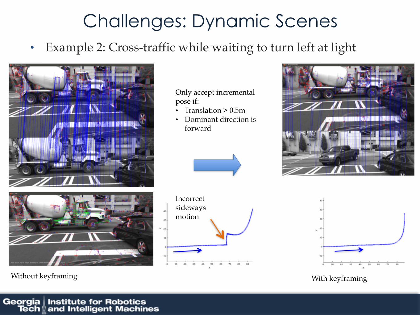
• Example 2: Cross-traffic while waiting to turn left at light
Only accept incremental pose if: • Translation > 0.5m • Dominant direction is
forward
Without keyframing With keyframing
Incorrect sideways motion
Challenges: Dynamic Scenes

• Parallelization of feature extraction and stereo matching steps allows real-time performance even in CPU-only implementation
Real-time performance
Mono Frame Queue
Stereo Frame Queue
Pose Recovery/RANSAC
…
Feature Extractor
Feature Extractor
Feature Extractor
Stereo Frame Queue
Stereo Matching
Stereo Matching

• Representative results on KITTI VO Benchmark • Average translational/rotational errors are very small • Accumulate over time, resulting in drift
Results on KITTI Benchmark

• Stereo Visual Odometry yields more than just a camera trajectory!
• Tracked landmarks form a sparse 3D point cloud of the environment
• Can be used as the basis for localization
What else do you get?

Intro Visual SLAM
Bundle Adjustment Factor Graphs Incremental Large-‐Scale
End
Outline
34
Intro Visual SLAM
Bundle Adjustment Factor Graphs Incremental Large-‐Scale
End

Motivation
• VO: just two frames -‐> R,t using 5-‐pt or 3-‐pt
• Can we do better? Bundle Adjustment -‐> VSLAM • Later: integrate IMU, other sensors

Objective Function
• refine VO by non-‐linear optimization
pij
T1w T2
w
Pjw

Two Views
• Unknowns: poses and points • Measurements pij: normalized (x,y), known K!
pij
T1w T2
w
Pjw

If we lived in a Linear World:

In a Linear World…
• Linear measurement function:
• …and objective function:
• Linear least-‐squares !
• Note: = 6D, = = 3D

Sparse Matters
• Rewrite as where

Normal Equations
• Least-‐squares criterion
• Take derivative, set to zero:
• Solve using cholmod, GTSAM… • In MATLAB: x=A\b

Generative Model
• Measurement Function, calibrated setting!
Rigid 3D transform to camera frame
Projection to intrinsic image coordinates

Taylor Expansion Epic Fail
• Taylor expansion?

Taylor Expansion Epic Fail
• Taylor expansion?
• Oops: ?
• T is a 4x4 matrix, but is over-‐parameterized! • T in SE(3): only 6DOF (3 rotation, 3 translation)

Tangent Spaces• An incremental change on a manifold can be introduced via
the notion of an n-‐dimensional tangent space at a • Sphere SO(2)
a
a==0

Tangent Spaces
• Provides local coordinate frame for manifold
a
0

SE(3): A Twist of Li(m)e
• Lie group = group + manifold – SE(3) is group! – SE(3) is 6DOF manifold embedded in R4*4
• For Lie groups, we have exponential maps:
• se<2> twist:

Exponential Map for SE(3)

Generators for SE(3)
Exponential map closed form:

Generalized Taylor Expansion
• Define f’(a) to satisfy:
=[0.2 0.3]

Taylor Expansion for Projection
• Projection: function of two variables,
2x6 2x3
)

Taylor Expansion for Projection
• Projection: function of two variables,
2x6 2x3

Gauss-‐Newton• Iteratively Linearize, solve normal equations on tangent space, update Lie group elements

Too much Freedom!
• A’A will be singular! 7DOF gauge freedom – Switch to 5DOF Essential Manifold – Use photogrammetry “inner constraints” – Add prior terms – Fuse in other sensors, e.g., IMU/GPS
SE(3) x SE(3) E
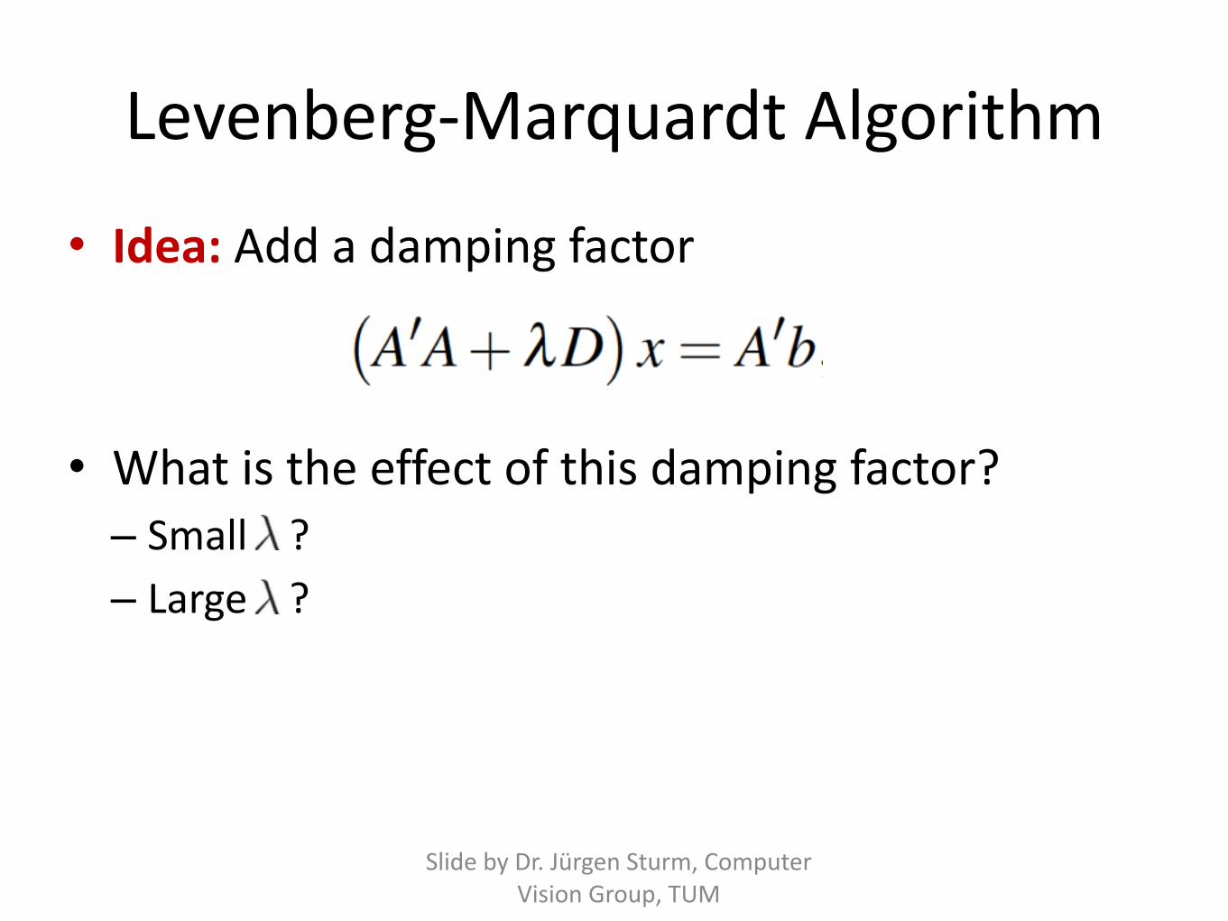
• Idea: Add a damping factor
• What is the effect of this damping factor? – Small ? – Large ?
Levenberg-‐Marquardt Algorithm
Slide by Dr. Jürgen Sturm, Computer Vision Group, TUM

Levenberg-‐Marquardt Algorithm
• Idea: Add a damping factor
• What is the effect of this damping factor? – Small à same as least squares – Large à steepest descent (with small step size)
• Algorithm – If error decreases, accept and reduce – If error increases, reject and increase
Slide by Dr. Jürgen Sturm, Computer Vision Group, TUM

Linearizing Re-‐projection Error
• Chain rule:

Linearizing Re-‐projection Error
• Chain rule:

Linearizing Re-‐projection Error
• Chain rule:

Linearizing Re-‐projection Error
• Chain rule:

Linearizing Re-‐projection Error
• Chain rule:

Intro Visual SLAM
Bundle Adjustment Factor Graphs Incremental Large-‐Scale
End
Outline
59
Intro Visual SLAM
Bundle Adjustment Factor Graphs Incremental Large-‐Scale
End

Frank Dellaert: Optimization in Factor Graphs for Fast and Scalable 3D Reconstruction and Mapping
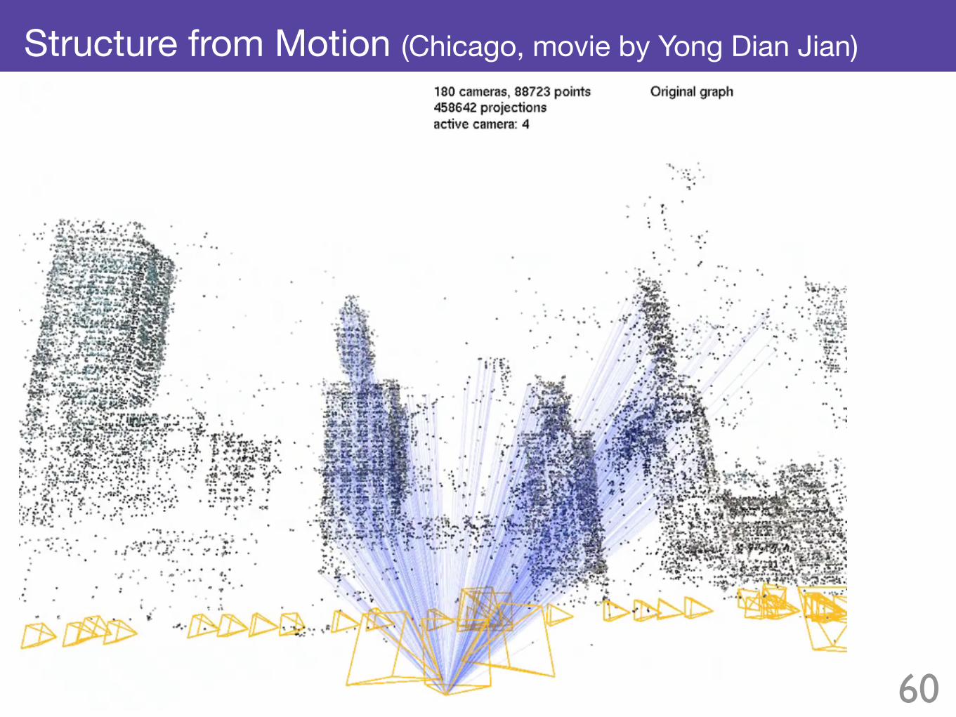
Structure from Motion (Chicago, movie by Yong Dian Jian)
60
Frank Dellaert: Optimization in Factor Graphs for Fast and Scalable 3D Reconstruction and Mapping
Structure from Motion (Chicago, movie by Yong Dian Jian)
60

Frank Dellaert: Optimization in Factor Graphs for Fast and Scalable 3D Reconstruction and Mapping
Boolean Satisfiability
61

Frank Dellaert: Optimization in Factor Graphs for Fast and Scalable 3D Reconstruction and Mapping
Boolean Satisfiability
M I
A H G
¬M ∨ I
M ∨ ¬I
M ∨ A
¬I ∨ H
¬A ∨ H ¬H ∨ G
61

Frank Dellaert: Optimization in Factor Graphs for Fast and Scalable 3D Reconstruction and Mapping
Boolean Satisfiability
M I
A H G
¬M ∨ I
M ∨ ¬I
M ∨ A
¬I ∨ H
¬A ∨ H ¬H ∨ G
Variables
61

Frank Dellaert: Optimization in Factor Graphs for Fast and Scalable 3D Reconstruction and Mapping
Boolean Satisfiability
M I
A H G
¬M ∨ I
M ∨ ¬I
M ∨ A
¬I ∨ H
¬A ∨ H ¬H ∨ G
Variables
Factors
61

Frank Dellaert: Optimization in Factor Graphs for Fast and Scalable 3D Reconstruction and Mapping
Boolean Satisfiability
M I
A H G
¬M ∨ I
M ∨ ¬I
M ∨ A
¬I ∨ H
¬A ∨ H ¬H ∨ G
Variables
Factors
Factor Graph
61

Frank Dellaert: Optimization in Factor Graphs for Fast and Scalable 3D Reconstruction and Mapping
Constraint Satisfaction
62

Frank Dellaert: Optimization in Factor Graphs for Fast and Scalable 3D Reconstruction and Mapping
Constraint Satisfaction
63
S
V
Y
NL
BC
N
NB
O
NT
M
Q

Frank Dellaert: Optimization in Factor Graphs for Fast and Scalable 3D Reconstruction and Mapping
Constraint Satisfaction
63
S
V
Y
NL
BC
N
NB
O
NT
M
Q

Frank Dellaert: Optimization in Factor Graphs for Fast and Scalable 3D Reconstruction and Mapping
Graphical Models
64
As a first step to perform inference, we take a Bayes net corresponding to the generative model andconvert it to a factor graph. However, because inference assumes known measurements Z, we drop them asvariables. Instead, the conditional densities P(zk|�k) on them are converted into likelihood factors
fk(�k)�= L(�k;zk) � P(zk|�k)
where zk acts as a parameter, not a variable. After this conversion, the factor graph represents the posteriorP(�|Z) as the product of the prior P(�) and the likelihood factors L(�k;zk),
P(�|Z) � P(�)�kL(�k;zk) = f0(�0)�
kfk(�k) (4.2)
where the factor f0 corresponding to the prior P(�) typically factors as well, depending on the application.
T
S
L
BE
X
Figure 4.3: Factor graph for examples in Figure 4.2.
Example 12. As an example, the Bayes net from Figure 4.2 is converted into the factor graph shown inFigure 4.3. Note that the observed variables do not appear as variables in the factor graph. Instead, theconstraint induced on the other variables by the observations is represented by corresponding factors.
4.2 Inference
4.2.1 Computations Supported by Factor Graphs
Converting to a factor graph with measurements as parameters yields a representation of the posteriorP(�|Z), given by Equation 4.2, and it is natural to ask what we can do with this.
Given any factor graph defining an unnormalized density f (�) we can easily evaluate it for any givenvalue of the parameters �. However, it is not obvious how to sample from the corresponding density
4.1 Representation
4.1.1 Bayesian Networks
A Bayesian network (Pearl, 1988) or Bayes net is a directed graphical model where the nodes representvariables x with conditional densities P(x|�) on them, and the edges indicate on which variables � we areconditioning. The joint probability density P(X) over all variables X = (x1 . . .xn) is then defined as theproduct of all the conditionals associated with the nodes:
P(X) =�iP(xi|�i) (4.1)
Bayes nets are an excellent language in which to think about and specify a generative model. They easilylend themselves to thinking about how a given measurement z depends on the parameters �. Importantly,they allow us to factor the joint density P(�,Z) into a product of simple factors. This is typically done byspecifying conditional densities of the form P(z|�), indicating that given the values for a subset � ⊂ � ofthe parameters, the measurement z is conditionally independent of all other parameters.
A
D
T
S
L
BE
X
Figure 4.2: Bayes nets for example in Figure 4.1. The observed variables are shown as square nodes.
Example 11. The Bayes net for our running example from Figure 4.1 is shown in Figure 4.2. In the figureI have indicated which of the variables are assumed to be measurements or observed variables. For theASIA example we will assume below that A and D were observed and that we want to do inference on theremaining variables, but other combinations of observations are possible. The joint probability for the ASIAexample can simply be read off from the graph:
P(A,S,T,L,E,B,X ,D) = P(A)P(S)P(T |A)P(L|S)P(E|T,L)P(B|S)P(X |E)P(D|E,B)
where the conditional probability tables are given in Table 4.1.
Frank Dellaert: Optimization in Factor Graphs for Fast and Scalable 3D Reconstruction and Mapping
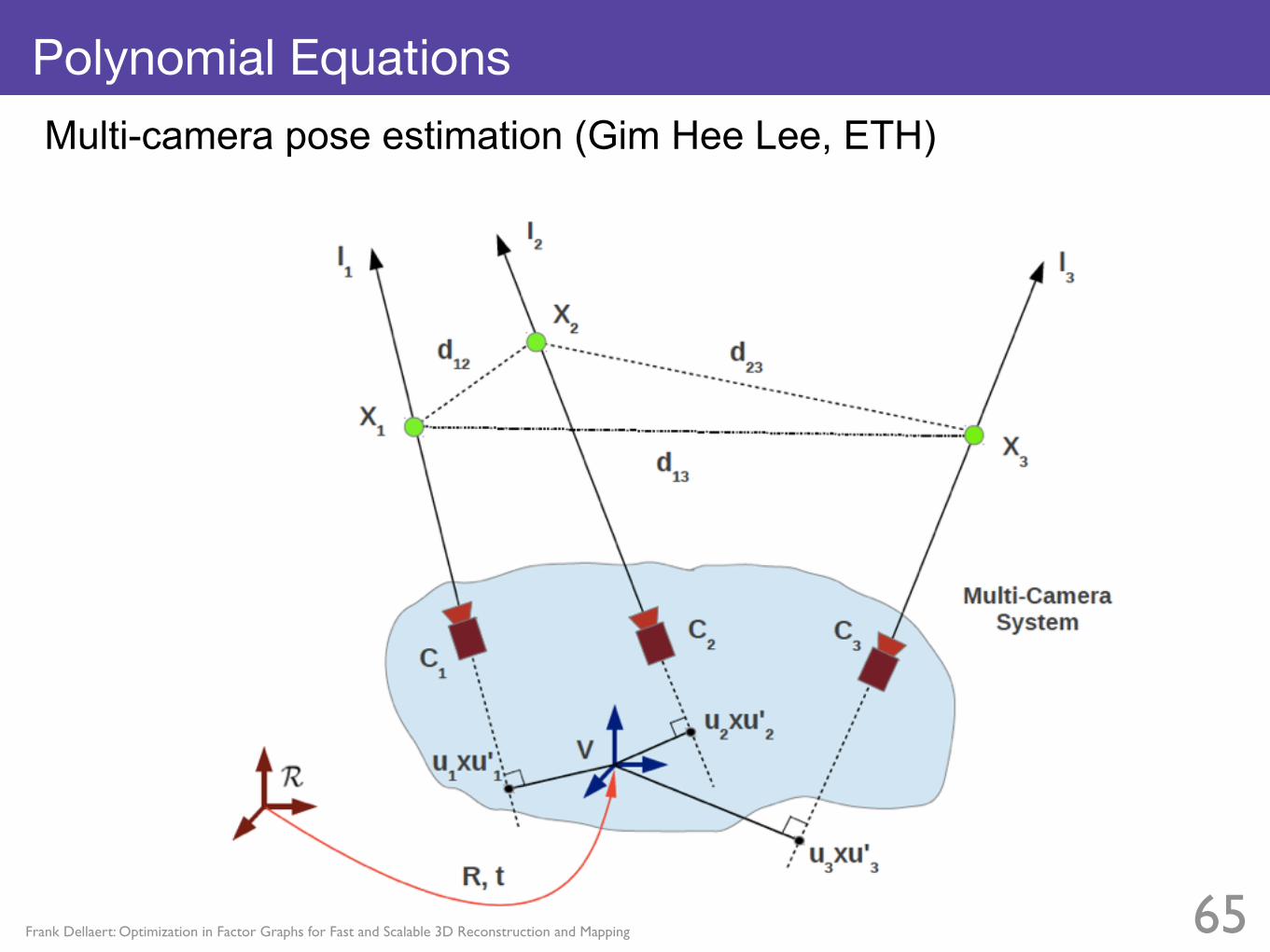
Polynomial Equations
65
Multi-camera pose estimation (Gim Hee Lee, ETH)

Frank Dellaert: Optimization in Factor Graphs for Fast and Scalable 3D Reconstruction and Mapping
Polynomial Equations
66
𝛾2
𝛾3𝛾1
Multi-camera pose estimation (Gim Hee Lee, ETH)

Frank Dellaert: Optimization in Factor Graphs for Fast and Scalable 3D Reconstruction and Mapping 67
Continuous Probability Densities
x0 x1 x2 xM...
lNl1 l2...
...
P(X,M) = k*
- E.g., Robot Trajectory
- Landmarks
- Measurements

Frank Dellaert: Optimization in Factor Graphs for Fast and Scalable 3D Reconstruction and Mapping 68
Simultaneous Localization and Mapping (SLAM)

Frank Dellaert: Optimization in Factor Graphs for Fast and Scalable 3D Reconstruction and Mapping 68
Simultaneous Localization and Mapping (SLAM)

Frank Dellaert: Optimization in Factor Graphs for Fast and Scalable 3D Reconstruction and Mapping 69
Factor Graph -> Smoothing and Mapping (SAM) !

Frank Dellaert: Optimization in Factor Graphs for Fast and Scalable 3D Reconstruction and Mapping 69
Factor Graph -> Smoothing and Mapping (SAM) !Variables are multivariate! Factors are non-linear!

Frank Dellaert: Optimization in Factor Graphs for Fast and Scalable 3D Reconstruction and Mapping 69
Factor Graph -> Smoothing and Mapping (SAM) !Variables are multivariate! Factors are non-linear!
Factors induce probability densities. -log P(x) = |E(x)|2

Full Bundle Adjustment
• Extend 2-‐frame case to multiple cameras:
• Factor graph representation:

Frank Dellaert: Optimization in Factor Graphs for Fast and Scalable 3D Reconstruction and Mapping
Structure from Motion (Chicago, movie by Yong Dian Jian)
71

Frank Dellaert: Optimization in Factor Graphs for Fast and Scalable 3D Reconstruction and Mapping
Structure from Motion (Chicago, movie by Yong Dian Jian)
71

Frank Dellaert
Nonlinear Least-Squares
72
Gaussian noise

Frank Dellaert
Nonlinear Least-Squares
Repeatedly solve linearized system (GN)
72
Gaussian noise

Frank Dellaert
Nonlinear Least-Squares
Repeatedly solve linearized system (GN)
72
A
b
Gaussian noise
poses points

Frank Dellaert: Optimization in Factor Graphs for Fast and Scalable 3D Reconstruction and Mapping 73
Gaussian Factor Graph == mxn Matrix
A
Frank Dellaert: Optimization in Factor Graphs for Fast and Scalable 3D Reconstruction and Mapping

Frank Dellaert
Solving the Linear Least-Squares System
74
A
Measurement Jacobian
Solve:

Frank Dellaert
Solving the Linear Least-Squares System
74
ATAA
Measurement Jacobian
Information matrix
Normal equations
Solve:

Frank Dellaert
Solving the Linear Least-Squares System
•Can we simply invert ATA to solve for x?
75
ATAInformation matrix
Normal equations

Frank Dellaert
Solving the Linear Least-Squares System
•Can we simply invert ATA to solve for x?
•Yes, but we shouldn’t… The inverse of ATA is dense -‐> O(n^3)
•Can do much better by takingadvantage of sparsity!
75
ATAInformation matrix
Normal equations
Frank Dellaert
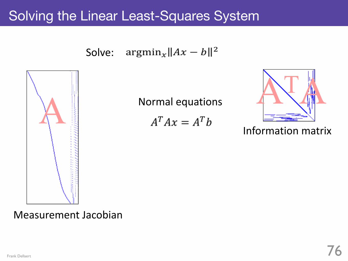
Solving the Linear Least-Squares System
76
ATAInformation matrix
Normal equations
Solve:
A
Measurement Jacobian

Frank Dellaert
Solving the Linear Least-Squares System
76
R
ATAInformation matrix
Square root information matrix
Normal equations
Matrix factorization
Solve:
A
Measurement Jacobian

Frank Dellaert
Matrix – Square Root Factorization
77
• QR on A: Numerically More Stable
• Cholesky on ATA: Faster
A QR R
Cholesky RATA

Frank Dellaert
Solving by Backsubstitution
After factorization (via Cholesky): RTR x = ATb
78

Frank Dellaert
Solving by Backsubstitution
After factorization (via Cholesky): RTR x = ATb
•Forward substitutionRTy = ATb, solve for y
78
RT

Frank Dellaert
Solving by Backsubstitution
After factorization (via Cholesky): RTR x = ATb
•Forward substitutionRTy = ATb, solve for y
•BacksubstitionR x = y, solve for x
78
RT
R

Frank Dellaert: Optimization in Factor Graphs for Fast and Scalable 3D Reconstruction and Mapping
Intel Dataset
79
910 poses, 4453 constraints, 45s or 49ms/step
(Olson, RSS 07: iterative equation solver, same ballpark)

Frank Dellaert: Optimization in Factor Graphs for Fast and Scalable 3D Reconstruction and Mapping
MIT Killian Court Dataset
80
1941 poses, 2190 constraints, 14.2s or 7.3ms/step
Frank Dellaert: Optimization in Factor Graphs for Fast and Scalable 3D Reconstruction and Mapping
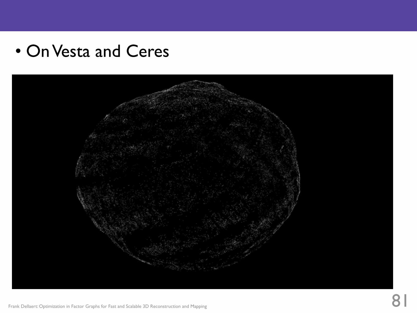
• On Vesta and Ceres
81

Frank Dellaert: Optimization in Factor Graphs for Fast and Scalable 3D Reconstruction and Mapping
• On Vesta and Ceres
81

Frank Dellaert: Inference in Factor Graphs, Tutorial at ICRA 2013
“Gaussian” Elimination?
82
The Nine Chapters on the Mathematical Art, 200 B.C.

Frank Dellaert: Inference in Factor Graphs, Tutorial at ICRA 2013
“Gaussian” Elimination?
82
The Nine Chapters on the Mathematical Art, 200 B.C.
Gauss re-invented elimination for determining the orbit of Ceres

Frank Dellaert: Inference in Factor Graphs, Tutorial at ICRA 2013
“Gaussian” Elimination?
82
The Nine Chapters on the Mathematical Art, 200 B.C.
Gauss re-invented elimination for determining the orbit of Ceres

Frank Dellaert: Optimization in Factor Graphs for Fast and Scalable 3D Reconstruction and Mapping 83
Variable Elimination
• Choose Ordering• Eliminate one node at a time
• Express node as function of adjacent nodes
x1 x2 x3
l1 l2
l1 l2 x1 x2 x3 xx x x x x x x x x x x x x

Frank Dellaert: Optimization in Factor Graphs for Fast and Scalable 3D Reconstruction and Mapping 83
Variable Elimination
• Choose Ordering• Eliminate one node at a time
• Express node as function of adjacent nodes
x1 x2 x3
l1 l2
Basis = Chain Rule ! e.g. P(l1,x1,x2)=P(l1|x1,x2)P(x1,x2)
P(l1,x1,x2)
l1 l2 x1 x2 x3 xx x x x x x x x x x x x x

Frank Dellaert: Optimization in Factor Graphs for Fast and Scalable 3D Reconstruction and Mapping
• Choose Ordering• Eliminate one node at a time
• Express node as function of adjacent nodes
x1 x2 x3
l1 l2l1
Small Example
84
P(l1|x1,x2)
P(x1,x2)
Basis = Chain Rule ! e.g. P(l1,x1,x2)=P(l1|x1,x2)P(x1,x2)
l1 l2 x1 x2 x3 x x x x x x x x x x x x x x
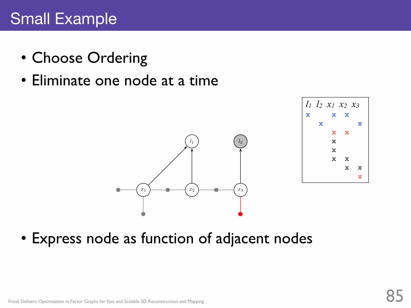
Frank Dellaert: Optimization in Factor Graphs for Fast and Scalable 3D Reconstruction and Mapping
• Choose Ordering• Eliminate one node at a time
• Express node as function of adjacent nodes
x1 x2 x3
l1 l2l2
Small Example
85
l1 l2 x1 x2 x3 x x x x x x x x x x x x x x

Frank Dellaert: Optimization in Factor Graphs for Fast and Scalable 3D Reconstruction and Mapping
• Choose Ordering• Eliminate one node at a time
• Express node as function of adjacent nodes
x1 x2 x3x1
l1 l2
Small Example
86
l1 l2 x1 x2 x3 x x x x x x x x x x x

Frank Dellaert: Optimization in Factor Graphs for Fast and Scalable 3D Reconstruction and Mapping
• Choose Ordering• Eliminate one node at a time
• Express node as function of adjacent nodes
x1 x2 x3x2
l1 l2
Small Example
87
l1 l2 x1 x2 x3 x x x x x x x x x x x

Frank Dellaert: Optimization in Factor Graphs for Fast and Scalable 3D Reconstruction and Mapping
• Choose Ordering• Eliminate one node at a time
• Express node as function of adjacent nodes
x1 x2 x3x3
l1 l2
Small Example
88
l1 l2 x1 x2 x3 x x x x x x x x x x

Frank Dellaert: Optimization in Factor Graphs for Fast and Scalable 3D Reconstruction and Mapping
x1 x2 x3x3
l1 l2
Small Example
89
• End-Result = Bayes Net ! l1 l2 x1 x2 x3 x x x x x x x x x x

Frank Dellaert: Optimization in Factor Graphs for Fast and Scalable 3D Reconstruction and Mapping
Polynomial Equations
90
Gim Hee Lee’s thesis: multi-camera pose estimation
𝛾2
𝛾3𝛾1
Frank Dellaert: Optimization in Factor Graphs for Fast and Scalable 3D Reconstruction and Mapping
Polynomial Equations
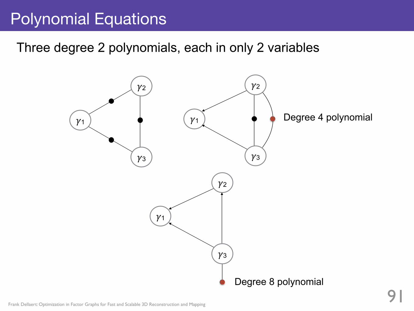
91
𝛾2
𝛾3
𝛾1 𝛾1
𝛾2
𝛾3
𝛾1
𝛾2
𝛾3
Three degree 2 polynomials, each in only 2 variables
Degree 8 polynomial
Degree 4 polynomial

Frank Dellaert: Optimization in Factor Graphs for Fast and Scalable 3D Reconstruction and Mapping
Elimination at work
92

Frank Dellaert: Optimization in Factor Graphs for Fast and Scalable 3D Reconstruction and Mapping
Elimination at work
92

Frank Dellaert: Optimization in Factor Graphs for Fast and Scalable 3D Reconstruction and Mapping
Elimination at work
93

Frank Dellaert: Optimization in Factor Graphs for Fast and Scalable 3D Reconstruction and Mapping
Elimination at work
93

Frank Dellaert: Optimization in Factor Graphs for Fast and Scalable 3D Reconstruction and Mapping 94
Elimination order is again CRUCIAL
• Order with least fill-in NP-complete to find
Square Root SAM: Simultaneous Location and Mapping via Square Root Information Smoothing, Frank Dellaert, Robotics: Science and Systems, 2005 Exploiting Locality by Nested Dissection For Square Root Smoothing and Mapping, Peter Krauthausen, Frank Dellaert, and Alexander Kipp, Robotics: Science and Systems, 2006

Frank Dellaert: Inference in Factor Graphs, Tutorial at ICRA 2013 95
Remember: Larger Example Factor Graph

Frank Dellaert: Inference in Factor Graphs, Tutorial at ICRA 2013 96
Eliminate Poses then LandmarksR

Frank Dellaert: Inference in Factor Graphs, Tutorial at ICRA 2013 97
Eliminate Landmarks then Poses

Frank Dellaert: Inference in Factor Graphs, Tutorial at ICRA 2013 98
Minimum Degree FillYields Chordal Graph. Chordal graph + order = directedR

Frank Dellaert: Inference in Factor Graphs, Tutorial at ICRA 2013 98
Minimum Degree FillYields Chordal Graph. Chordal graph + order = directedR

The importance of being Ordered
500 Landmarks, 1000 steps, many loops

The importance of being Ordered
500 Landmarks, 1000 steps, many loops

The importance of being Ordered
500 Landmarks, 1000 steps, many loops

The importance of being Ordered
500 Landmarks, 1000 steps, many loops
Bottom line: even a tiny amount of domain knowledge helps.

The importance of being Ordered
500 Landmarks, 1000 steps, many loops
Bottom line: even a tiny amount of domain knowledge helps.
Bottom line 2: this is EXACT !!!

Frank Dellaert: Optimization in Factor Graphs for Fast and Scalable 3D Reconstruction and Mapping
Approximate Minimum Degree
100

Frank Dellaert: Optimization in Factor Graphs for Fast and Scalable 3D Reconstruction and Mapping
Approximate Minimum Degree
100
Frank Dellaert: Optimization in Factor Graphs for Fast and Scalable 3D Reconstruction and Mapping
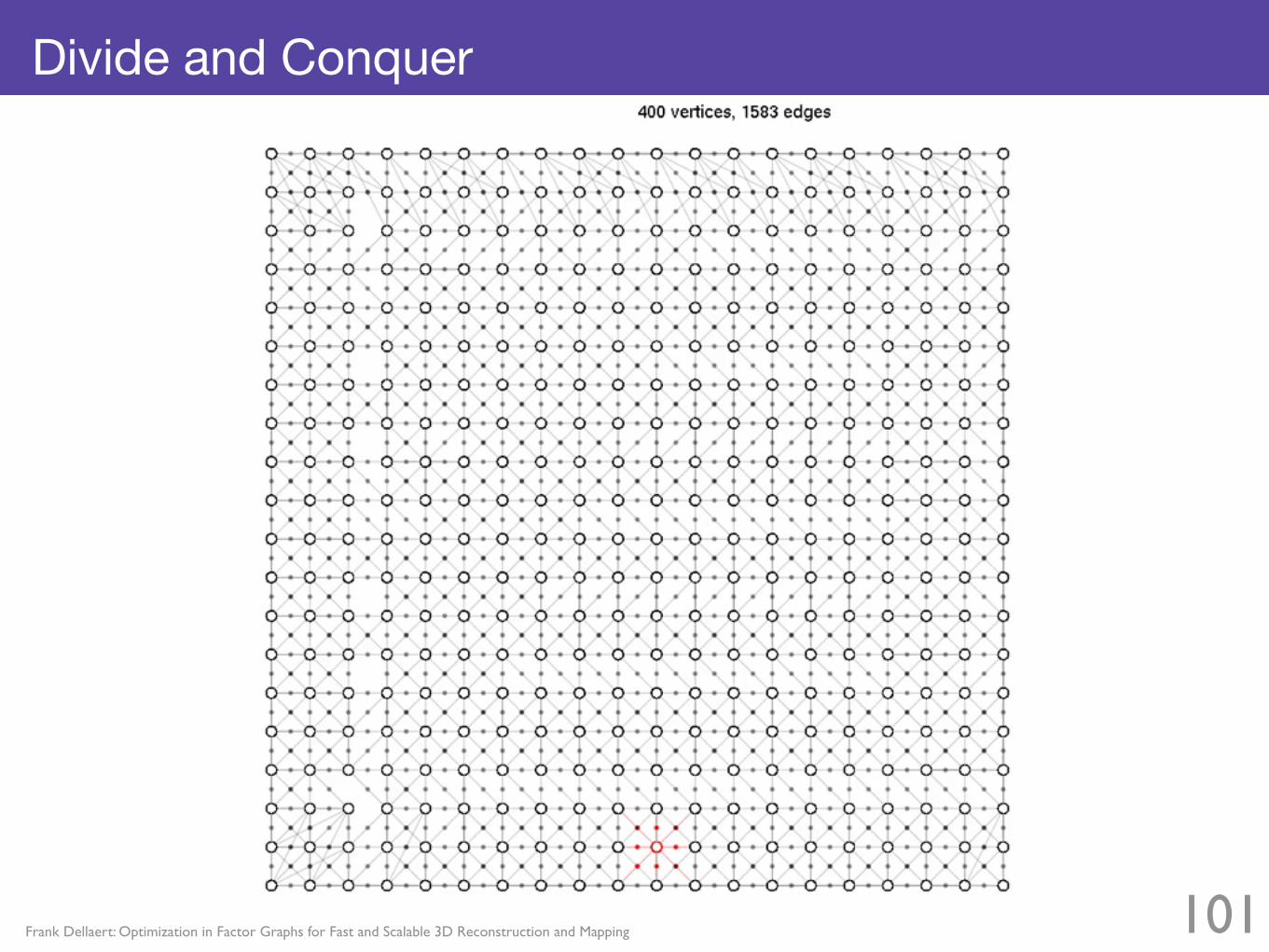
Divide and Conquer
101

Frank Dellaert: Optimization in Factor Graphs for Fast and Scalable 3D Reconstruction and Mapping
Divide and Conquer
101

Frank Dellaert: Optimization in Factor Graphs for Fast and Scalable 3D Reconstruction and Mapping 102
St. Peter’s Basilica, Rome
Data Courtesy Microsoft Research
Kai Ni, Drew Steedly, and Frank Dellaert, Out-of-Core Bundle Adjustment for Large-Scale 3D Reconstruction, IEEE International Conference on Computer Vision (ICCV), 2007.

Frank Dellaert: Optimization in Factor Graphs for Fast and Scalable 3D Reconstruction and Mapping
Nested Dissection (but good separators are hard)
103

Frank Dellaert: Optimization in Factor Graphs for Fast and Scalable 3D Reconstruction and Mapping
Nested Dissection (but good separators are hard)
103

Frank Dellaert: Optimization in Factor Graphs for Fast and Scalable 3D Reconstruction and Mapping
Nested-Dissection for SFM: Hyper-SFM
104Kai Ni, and Frank Dellaert, HyperSfM, IEEE International Conference on 3D Imaging, Modeling, Processing, Visualization and Transmission (3DIMPVT), 2012.

Intro Visual SLAM
Bundle Adjustment Factor Graphs Incremental Large-‐Scale
End
Outline
105
Intro Visual SLAM
Bundle Adjustment Factor Graphs Incremental Large-‐Scale
End

Michael Kaess‹#› CVPR14: Visual SLAM Tutorial
The Mapping Problem (t=0)
Robot Onboard sensors: – Wheel odometry – Inertial measurement unit (gyro, accelerometer)
– Sonar – Laser range finder – Camera – RGB-‐D sensors

Michael Kaess‹#› CVPR14: Visual SLAM Tutorial
The Mapping Problem (t=0)
Robot
Landmark
LandmarkMeasurement
Onboard sensors: – Wheel odometry – Inertial measurement unit (gyro, accelerometer)
– Sonar – Laser range finder – Camera – RGB-‐D sensors
Michael Kaess‹#› CVPR14: Visual SLAM Tutorial
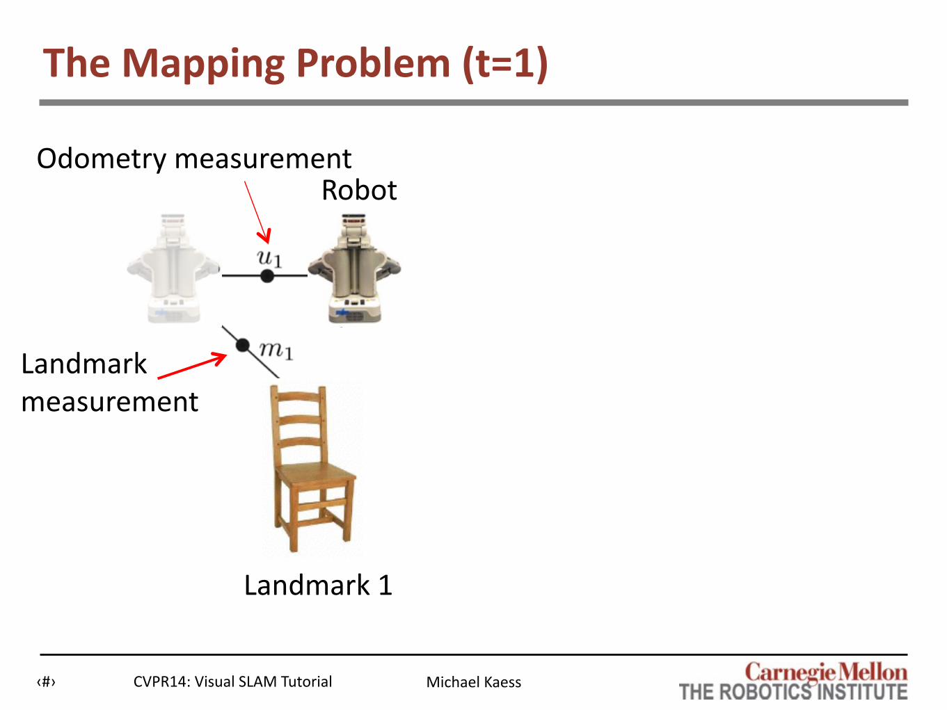
The Mapping Problem (t=1)
Robot
Landmark 1
Odometry measurement
Landmarkmeasurement

Michael Kaess‹#› CVPR14: Visual SLAM Tutorial
The Mapping Problem (t=1)
Robot
Landmark 1 Landmark 2
Odometry measurement
Landmarkmeasurement

Michael Kaess‹#› CVPR14: Visual SLAM Tutorial
The Mapping Problem (t=n-‐1)
Robot
Landmark 1 Landmark 2
Odometry measurement
Landmarkmeasurement

Michael Kaess‹#› CVPR14: Visual SLAM Tutorial
The Mapping Problem (t=n)
Odometry measurement
Landmarkmeasurement

Michael Kaess‹#› CVPR14: Visual SLAM Tutorial
The Mapping Problem (t=n)
Odometry measurement
Landmarkmeasurement
Mapping problem is incremental !

Michael Kaess‹#› CVPR14: Visual SLAM Tutorial
Factor Graph Representation
Robot pose
Landmark positionLandmarkmeasurement
Odometry measurement

Michael Kaess‹#› CVPR14: Visual SLAM Tutorial
Factor Graph Representation
Pose
PointPoint measurement

Michael Kaess‹#› CVPR14: Visual SLAM Tutorial
Full Bundle Adjustment
•Graph grows with time: – Have to solve a sequence of increasingly larger BA problems – Will become too expensive even for sparse Cholesky
F. Dellaert and M. Kaess, “Square Root SAM: Simultaneous localization and mapping via square root information smoothing,” IJRR 2006
From Strasdat et al, 2011 IVC “Visual SLAM: Why filter?”

Michael Kaess‹#› CVPR14: Visual SLAM Tutorial
Keyframe Bundle Adjustment
•Drop subset of poses to reduce density/complexity •Only retain “keyframes” necessary for good map
• Complexity still grows with time, just slower

Michael Kaess‹#› CVPR14: Visual SLAM Tutorial
Filter
•Marginalize out previous poses– Extended Kalman Filter (EKF)
• Problems when used for Visual SLAM:

Michael Kaess‹#› CVPR14: Visual SLAM Tutorial
Filter
•Marginalize out previous poses– Extended Kalman Filter (EKF)
• Problems when used for Visual SLAM:– All points become fully connected -‐> expensive– Relinearization not possible -‐> inconsistent
Michael Kaess‹#› CVPR14: Visual SLAM Tutorial
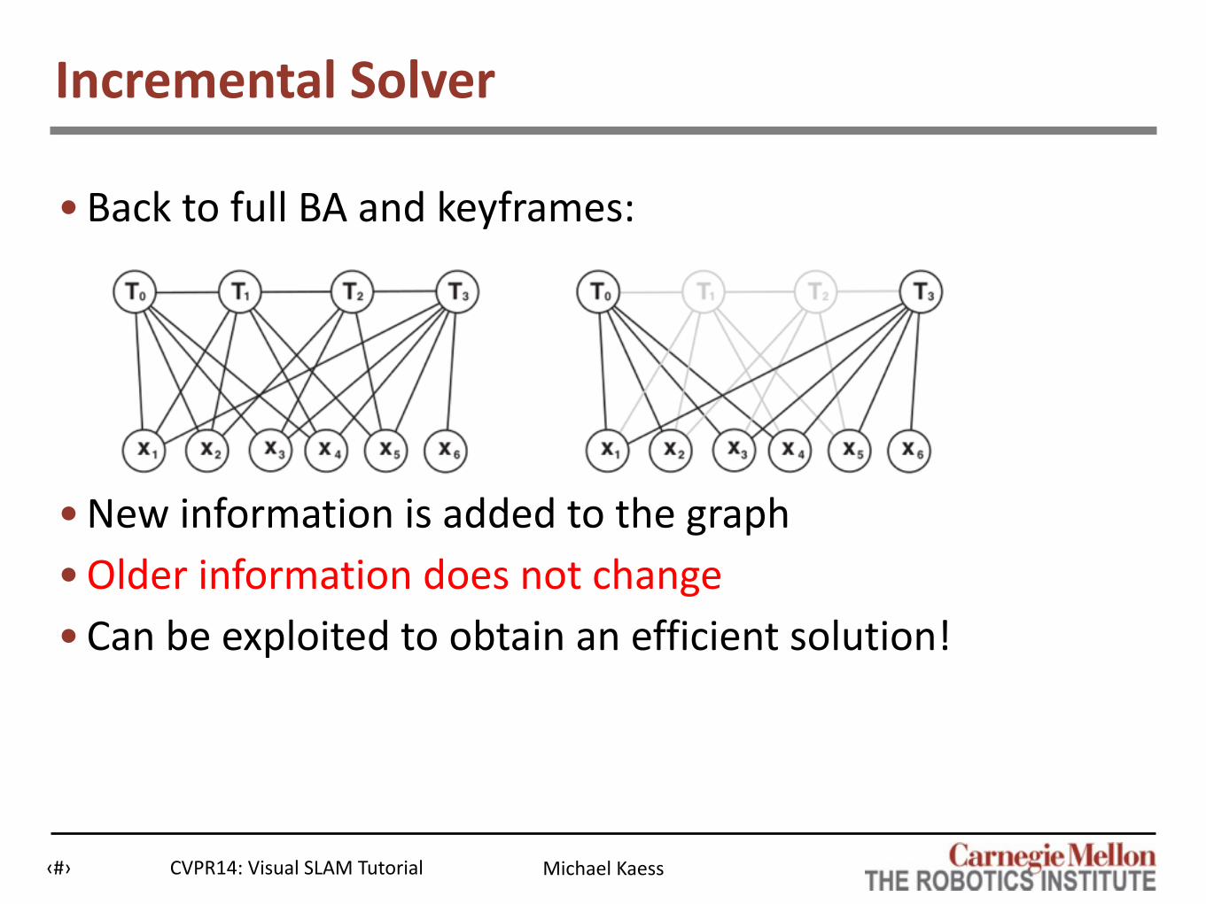
Incremental Solver
•Back to full BA and keyframes:
•New information is added to the graph •Older information does not change • Can be exploited to obtain an efficient solution!

Michael Kaess‹#› CVPR14: Visual SLAM Tutorial
Incremental Smoothing and Mapping (iSAM)
Solving a growing system:– R factor from previous step– How do we add new measurements? R
[Kaess et al., TRO 08]

Michael Kaess‹#› CVPR14: Visual SLAM Tutorial
Incremental Smoothing and Mapping (iSAM)
Solving a growing system:– R factor from previous step– How do we add new measurements?
Key idea:– Append to existing matrix factorization
R
New measurements -‐>
[Kaess et al., TRO 08]

Michael Kaess‹#› CVPR14: Visual SLAM Tutorial
Incremental Smoothing and Mapping (iSAM)
Solving a growing system:– R factor from previous step– How do we add new measurements?
Key idea:– Append to existing matrix factorization– “Repair” using Givens rotations
R
R’
New measurements -‐>
[Kaess et al., TRO 08]

Michael Kaess‹#› CVPR14: Visual SLAM Tutorial
Update and solution are O(1)
[Kaess et al., TRO 08]
Incremental Smoothing and Mapping (iSAM)

Michael Kaess‹#› CVPR14: Visual SLAM Tutorial
Update and solution are O(1)
[Kaess et al., TRO 08]
Incremental Smoothing and Mapping (iSAM)

Michael Kaess‹#› CVPR14: Visual SLAM Tutorial
Update and solution are O(1)
Are we done?BA is nonlinear…iSAM requires periodic batch factorization to relinearizeNot O(1), we need iSAM2!
[Kaess et al., TRO 08]
Incremental Smoothing and Mapping (iSAM)

Michael Kaess‹#› CVPR14: Visual SLAM Tutorial
Update and solution are O(1)
Are we done?BA is nonlinear…iSAM requires periodic batch factorization to relinearizeNot O(1), we need iSAM2!
[Kaess et al., TRO 08]
Incremental Smoothing and Mapping (iSAM)

Michael Kaess‹#› CVPR14: Visual SLAM Tutorial
Fixed-‐lag Smoothing
•Marginalize out all but last n poses and connected landmarks– Relinearization possible
plus some fill-‐in

Michael Kaess‹#› CVPR14: Visual SLAM Tutorial
Fixed-‐lag Smoothing
•Marginalize out all but last n poses and connected landmarks– Relinearization possible
• Linear case
Fixed lag
Cut here to marginalize
plus some fill-‐in

Michael Kaess‹#› CVPR14: Visual SLAM Tutorial
Fixed-‐lag Smoothing
•Marginalize out all but last n poses and connected landmarks– Relinearization possible
• Linear case•Nonlinear: need iSAM2
Fixed lag
Cut here to marginalize
plus some fill-‐in

Michael Kaess‹#› CVPR14: Visual SLAM Tutorial
Matrix vs. Graph
Measurement JacobianFactor Graph
x0 x1 x2 xM...
lNl1 l2...
...A

Michael Kaess‹#› CVPR14: Visual SLAM Tutorial
Matrix vs. Graph
Measurement JacobianFactor Graph
Information MatrixMarkov Random Field
x0 x1 x2 xM...
lNl1 l2...
...
x0 x1 x2 xM...
lNl1 l2...
...A
ATA

Michael Kaess‹#› CVPR14: Visual SLAM Tutorial
Matrix vs. Graph
Measurement JacobianFactor Graph
Information MatrixMarkov Random Field
Square Root Inf. Matrix
x0 x1 x2 xM...
lNl1 l2...
...
x0 x1 x2 xM...
lNl1 l2...
...
R
A
ATA
?

Michael Kaess‹#› CVPR14: Visual SLAM Tutorial
iSAM2: Bayes Tree Data Structure
Step 1
[Kaess et al., IJRR 12]

Michael Kaess‹#› CVPR14: Visual SLAM Tutorial
iSAM2: Bayes Tree Data Structure
Step 2: Find cliques in reverse elimination order:
Step 1
[Kaess et al., IJRR 12]

Michael Kaess‹#› CVPR14: Visual SLAM Tutorial
iSAM2: Bayes Tree Data Structure
Step 2: Find cliques in reverse elimination order:
Step 1
[Kaess et al., IJRR 12]

Michael Kaess‹#› CVPR14: Visual SLAM Tutorial
iSAM2: Bayes Tree Data Structure
Step 2: Find cliques in reverse elimination order:
Step 1
[Kaess et al., IJRR 12]

Michael Kaess‹#› CVPR14: Visual SLAM Tutorial
iSAM2: Bayes Tree Data Structure
Step 2: Find cliques in reverse elimination order:
Step 1
[Kaess et al., IJRR 12]

Michael Kaess‹#› CVPR14: Visual SLAM Tutorial
iSAM2: Bayes Tree Data Structure
Step 2: Find cliques in reverse elimination order:
Step 1
[Kaess et al., IJRR 12]

Michael Kaess‹#› CVPR14: Visual SLAM Tutorial
iSAM2: Bayes Tree Data Structure
Step 2: Find cliques in reverse elimination order:
Step 1
[Kaess et al., IJRR 12]

Michael Kaess‹#› CVPR14: Visual SLAM Tutorial
iSAM2: Bayes Tree Example
Manhattan dataset (Olson)
[Kaess et al., IJRR 12]

Michael Kaess‹#› CVPR14: Visual SLAM Tutorial
iSAM2: Bayes Tree Example
How to update with new measurements / add variables?
Manhattan dataset (Olson)
[Kaess et al., IJRR 12]

Michael Kaess‹#› CVPR14: Visual SLAM Tutorial
iSAM2: Updating the Bayes Tree
Add new factor between x1 and x3
[Kaess et al., IJRR 12]

Michael Kaess‹#› CVPR14: Visual SLAM Tutorial
iSAM2: Updating the Bayes Tree
Add new factor between x1 and x3
[Kaess et al., IJRR 12]

Michael Kaess‹#› CVPR14: Visual SLAM Tutorial
iSAM2: Updating the Bayes Tree
Add new factor between x1 and x3
[Kaess et al., IJRR 12]

Michael Kaess‹#› CVPR14: Visual SLAM Tutorial
iSAM2: Updating the Bayes Tree
Add new factor between x1 and x3
[Kaess et al., IJRR 12]

Michael Kaess‹#› CVPR14: Visual SLAM Tutorial
iSAM2: Bayes Tree for Manhattan Sequence[Kaess et al., IJRR 12]

Michael Kaess‹#› CVPR14: Visual SLAM Tutorial
iSAM2: Bayes Tree for Manhattan Sequence[Kaess et al., IJRR 12]

Intro Visual SLAM
Bundle Adjustment Factor Graphs Incremental Large-‐Scale
End
Outline
126
Intro Visual SLAM
Bundle Adjustment Factor Graphs Incremental Large-‐Scale
End
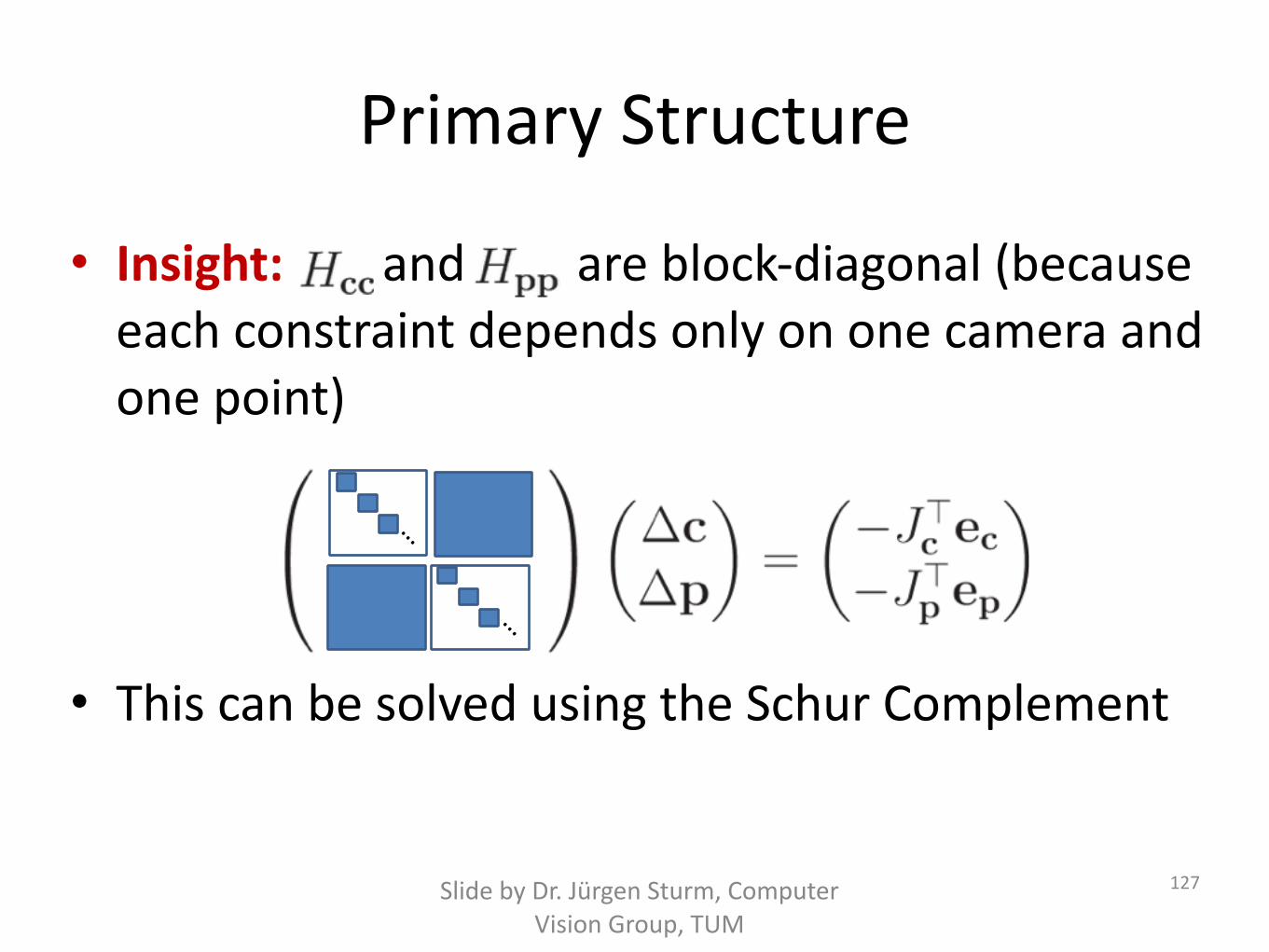
Primary Structure
• Insight: and are block-‐diagonal (because each constraint depends only on one camera and one point)
• This can be solved using the Schur Complement
127
…
…
Slide by Dr. Jürgen Sturm, Computer Vision Group, TUM

Schur Complement
• Given: Linear system
• If D is invertible, then (using Gauss elimination)
• Reduced complexity? • A: not in theory! But cache-‐friendly, repeatable
Slide by Dr. Jürgen Sturm, Computer Vision Group, TUM

Frank Dellaert: Optimization in Factor Graphs for Fast and Scalable 3D Reconstruction and Mapping
Of Eiffel Towers....
129

Frank Dellaert: Optimization in Factor Graphs for Fast and Scalable 3D Reconstruction and Mapping
Of Eiffel Towers....
129

Frank Dellaert: Optimization in Factor Graphs for Fast and Scalable 3D Reconstruction and Mapping
Iterative Methods
Better than direct methods for large problems because theyPerform only simple operations and no variable eliminationRequire constant (linear) memory
But they may converge slowlywhen the problem is ill-conditioned
The conjugate gradient method: The convergence speed is related tothe condition number (AtA) = �
max
/�min
13 / 40���130Frank Dellaert: Optimization in Factor Graphs for Fast and Scalable 3D Reconstruction and Mapping
Frank Dellaert: Optimization in Factor Graphs for Fast and Scalable 3D Reconstruction and Mapping
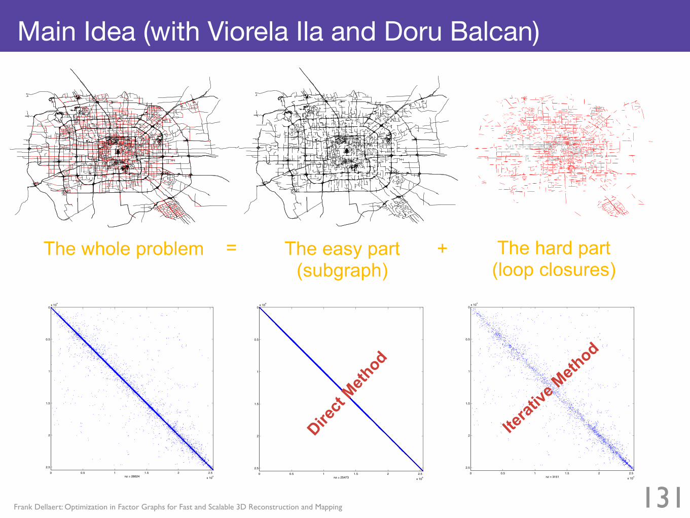
Main Idea (with Viorela Ila and Doru Balcan)
0 0.5 1 1.5 2 2.5
x 104
0
0.5
1
1.5
2
2.5
x 104
nz = 3151
0 0.5 1 1.5 2 2.5
x 104
0
0.5
1
1.5
2
2.5
x 104
nz = 286240 0.5 1 1.5 2 2.5
x 104
0
0.5
1
1.5
2
2.5
x 104
nz = 25473
The whole problem The easy part (subgraph)
The hard part (loop closures)
Direct
Method
Iterat
ive M
ethod
= +
131
Frank Dellaert: Optimization in Factor Graphs for Fast and Scalable 3D Reconstruction and Mapping
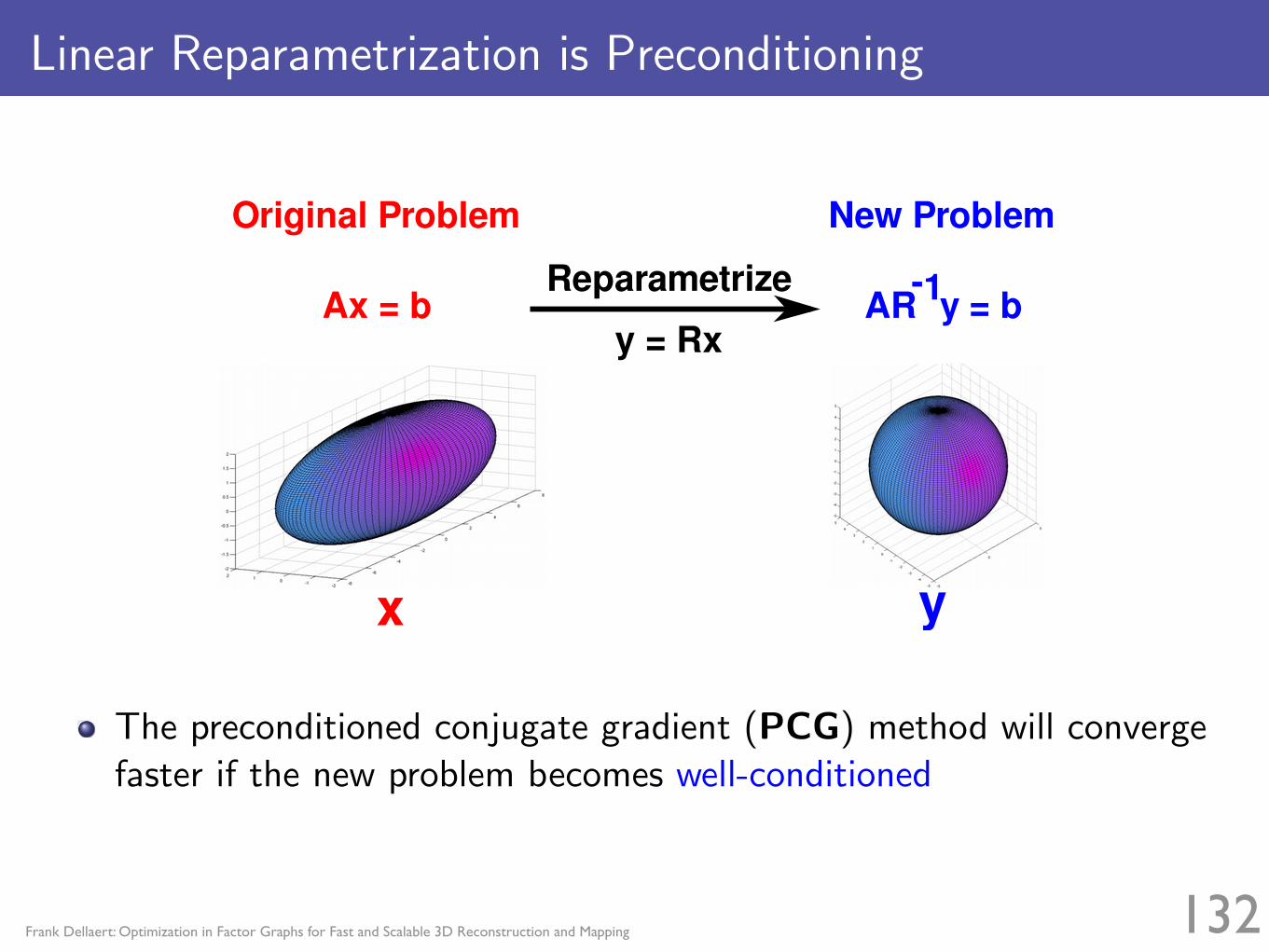
Linear Reparametrization is Preconditioning
�������������
������������
����� ���
��������
� �
������ ������
The preconditioned conjugate gradient (PCG) method will convergefaster if the new problem becomes well-conditioned
18 / 40���132Frank Dellaert: Optimization in Factor Graphs for Fast and Scalable 3D Reconstruction and Mapping

Frank Dellaert: Optimization in Factor Graphs for Fast and Scalable 3D Reconstruction and Mapping
Original, max
133

Frank Dellaert: Optimization in Factor Graphs for Fast and Scalable 3D Reconstruction and Mapping
Original, max
133

Frank Dellaert: Optimization in Factor Graphs for Fast and Scalable 3D Reconstruction and Mapping
Preconditioner
134

Frank Dellaert: Optimization in Factor Graphs for Fast and Scalable 3D Reconstruction and Mapping
Preconditioner
134

Frank Dellaert: Optimization in Factor Graphs for Fast and Scalable 3D Reconstruction and Mapping
Preconditioned, max
135

Frank Dellaert: Optimization in Factor Graphs for Fast and Scalable 3D Reconstruction and Mapping
Preconditioned, max
135

Frank Dellaert: Optimization in Factor Graphs for Fast and Scalable 3D Reconstruction and Mapping
Illustration with Real Data
Reconstruction results of a street scene dataset [Agarwal et al. ECCV’10]
Solution to a sparse subgraphAn approximated solutionE�cient to compute
Solution to the entire graphThe optimal solutionExpensive to compute directly
Use the subgraph solution to reparametrize the original problem21 / 40���136Frank Dellaert: Optimization in Factor Graphs for Fast and Scalable 3D Reconstruction and Mapping
Yong-Dian Jian, Doru C. Balcan and Frank DellaertGeneralized Subgraph Preconditioners for Large-Scale Bundle Adjustment Proceedings of 13th International Conference on Computer Vision (ICCV), Barcelona, 2011

Frank Dellaert: Optimization in Factor Graphs for Fast and Scalable 3D Reconstruction and Mapping
Solution from Subgraph Solution from the Original Graph
Data from Noah Snavely
Notre Dame
137

Frank Dellaert: Optimization in Factor Graphs for Fast and Scalable 3D Reconstruction and Mapping
Solution from Subgraph Solution from the Original Graph
Data from Sameer Agarwal
Piazza San Marco
138

Frank Dellaert: Optimization in Factor Graphs for Fast and Scalable 3D Reconstruction and Mapping
Results (3)
The condition numbers of the preconditioned systems
source Original SPCG Jacobi GSP-3
D-15 5.58e+21 1.87e+06 5.94e+04 4.36e+03
V-02 6.54e+21 6.46e+09 6.35e+05 1.38e+05
F-01 3.68e+11 1.92e+08 7.54e+06 8.71e+05
The original condition numbers are very large
GSP-3 has consistently smaller condition numbers
39 / 40���139Frank Dellaert: Optimization in Factor Graphs for Fast and Scalable 3D Reconstruction and Mapping

Frank Dellaert
State of the art = Schur Complement + Iterative
• Condition number of reduced camera matrix is already much lower
• Cluster based on co-visibility of features• Pre-conditioner = tree of clusters• Visibility Based Preconditioning, Kushal & Agarwal,
CVPR 2012, Experimental in Ceres140

Intro Visual SLAM
Bundle Adjustment Factor Graphs Incremental Large-‐Scale
End
Outline
141
Intro Visual SLAM
Bundle Adjustment Factor Graphs Incremental Large-‐Scale
End

Three Questions
• What is an exponential map? • What is a good elimination order for BA? • Which system has a high condition number?

SFM/BA Packages• SBA: pioneer • Google Ceres: great at large-‐scale BA • GTSAM (Georgia Tech Smoothing and Mapping)
– Has iSAM, iSAM2 (later), ideal for sensor fusion – Factor-‐graph based throughout:

LagoLinear Approximation for Graph Optimization
Smart FactorsMulti-‐threading
NEW RELEASE: GTSAM 3.1 Georgia Tech Smoothing And Mapping
Download: collab.cc.gatech.edu/borg/gtsam
Includes numerous performance improvements and features: • Multi-‐threading with TBB (funded by DARPA) • Smart Projection Factors for SfM • LAGO Initialization for planar SLAM (Luca Carlone et. al)


