31
1 Lecture 08: G x E: Genotype-by- environment interactions: Standard methods Bruce Walsh lecture notes Tucson Winter Institute 9 - 11 Jan 2013
| Date post: | 30-Aug-2018 |
| Category: |
Documents |
| Upload: | truongngoc |
| View: | 215 times |
| Download: | 0 times |

1
Lecture 08:G x E: Genotype-by-
environment interactions:Standard methods
Bruce Walsh lecture notesTucson Winter Institute
9 - 11 Jan 2013

2
G x E• Introduction to G x E
– Basics of G x E
– G x E is a correlated characters problem
– Finlay-Wilkinson regressions
• SVD-based methods– The singular value decomposition (SVD)
– AMMI models
• Factorial regressions
3
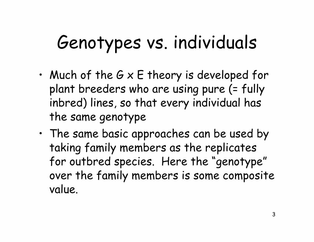
Genotypes vs. individuals
• Much of the G x E theory is developed forplant breeders who are using pure (= fullyinbred) lines, so that every individual hasthe same genotype
• The same basic approaches can be used bytaking family members as the replicatesfor outbred species. Here the “genotype”over the family members is some compositevalue.

4
Yield in Environment 2
Yield in Environment 1
Genotype 1
Genotype 2
G11
G12
G21
G22
E1
E2
E2E1 G1 G2
Ei = mean value in environment i
Overall means
5
G11 G12G21 G22
E2E1 G1 G2
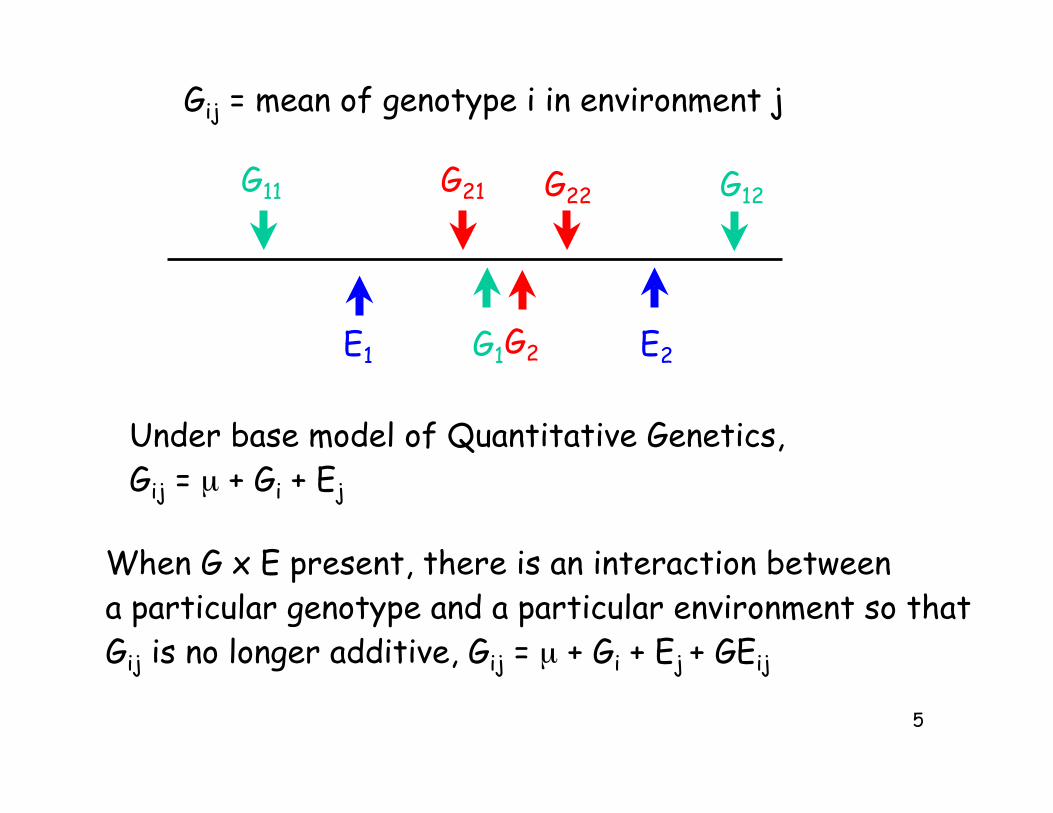
Gij = mean of genotype i in environment j
Under base model of Quantitative Genetics,Gij = µ + Gi + Ej
When G x E present, there is an interaction betweena particular genotype and a particular environment so thatGij is no longer additive, Gij = µ + Gi + Ej + GEij

6
G11 G12G21 G22
E2E1 G1 G2
µ
Components measured as deviations from the mean µ
GEij = gij - gi - ej
e2e1
g1
g11g12
g2
g22g21

7
Which genotype is the best?
G11 G12G21 G22
E2E1 G1 G2
Depends: If the genotypes are grown in both environments,G2 has a higher mean
If the genotypes are only grown in environment 1, G2 has a higher mean
If the genotypes are only grown in environment 2, G1 has a higher mean
8
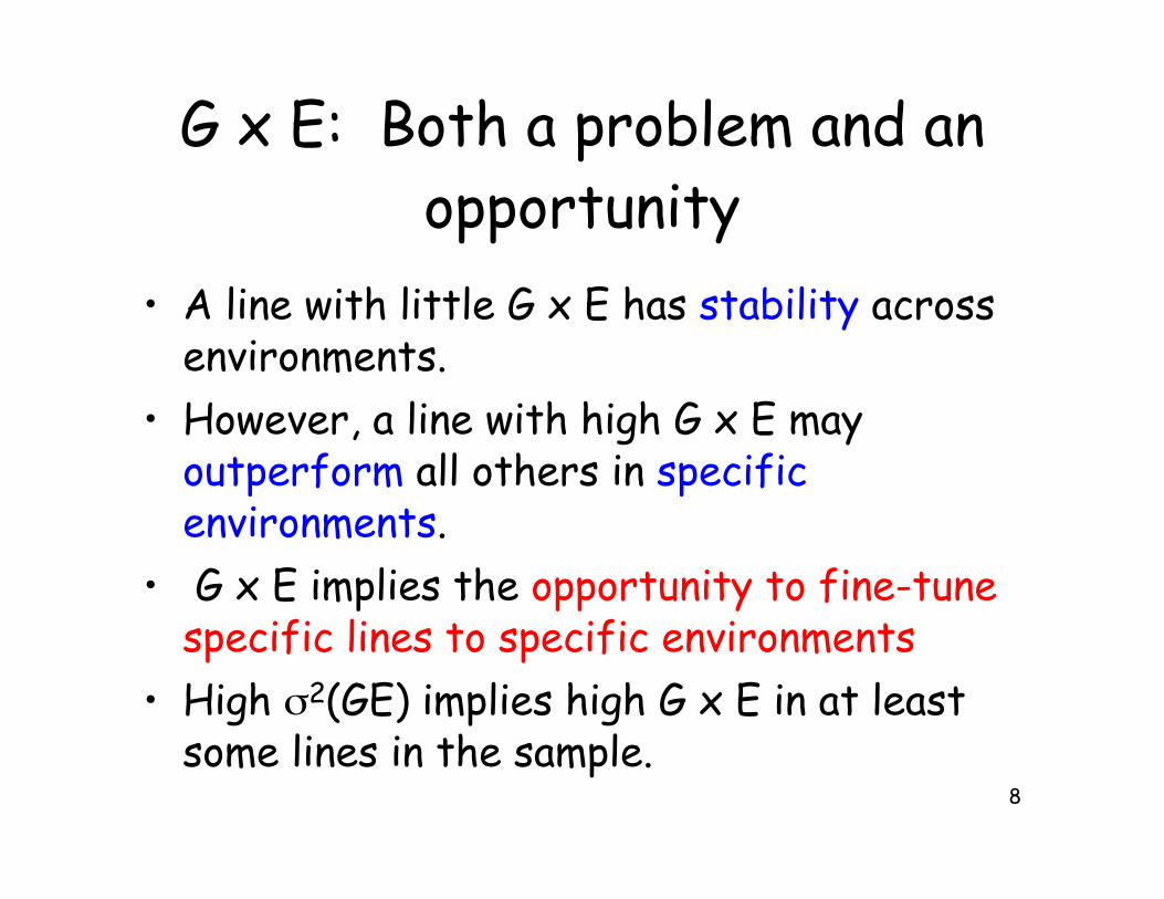
G x E: Both a problem and anopportunity
• A line with little G x E has stability acrossenvironments.
• However, a line with high G x E mayoutperform all others in specificenvironments.
• G x E implies the opportunity to fine-tunespecific lines to specific environments
• High !2(GE) implies high G x E in at leastsome lines in the sample.

9
G x E is Both a Challenge and an Opportunity
High G x E = potential for locally-adapted linesHigh G x E = poor stability across environments

10
G x E can be generated by either differences in theadditive variance over environments or by lack of perfect genetic correlation among environments

11
Major vs. minor environments• An identical genotype will display slightly different traits
values even over apparently identical environments due tomicro-environmental variation and developmental noise
• However, macro-environments (such as different locationsor different years <such as a wet vs. a dry year>) can showsubstantial variation, and genotypes (pure lines) maydifferentially perform over such macro-environments (G xE).
• Problem: The mean environment of a location may besomewhat predictable (e.g., corn in the tropics vs. temperateNorth American), but year-to-year variation at the samelocation is essentially unpredictable.
• Decompose G x E into components
– G x Elocations + G x Eyears + G x Eyears x locations
– Ideal: strong G x E over locations, high stability over years.
12
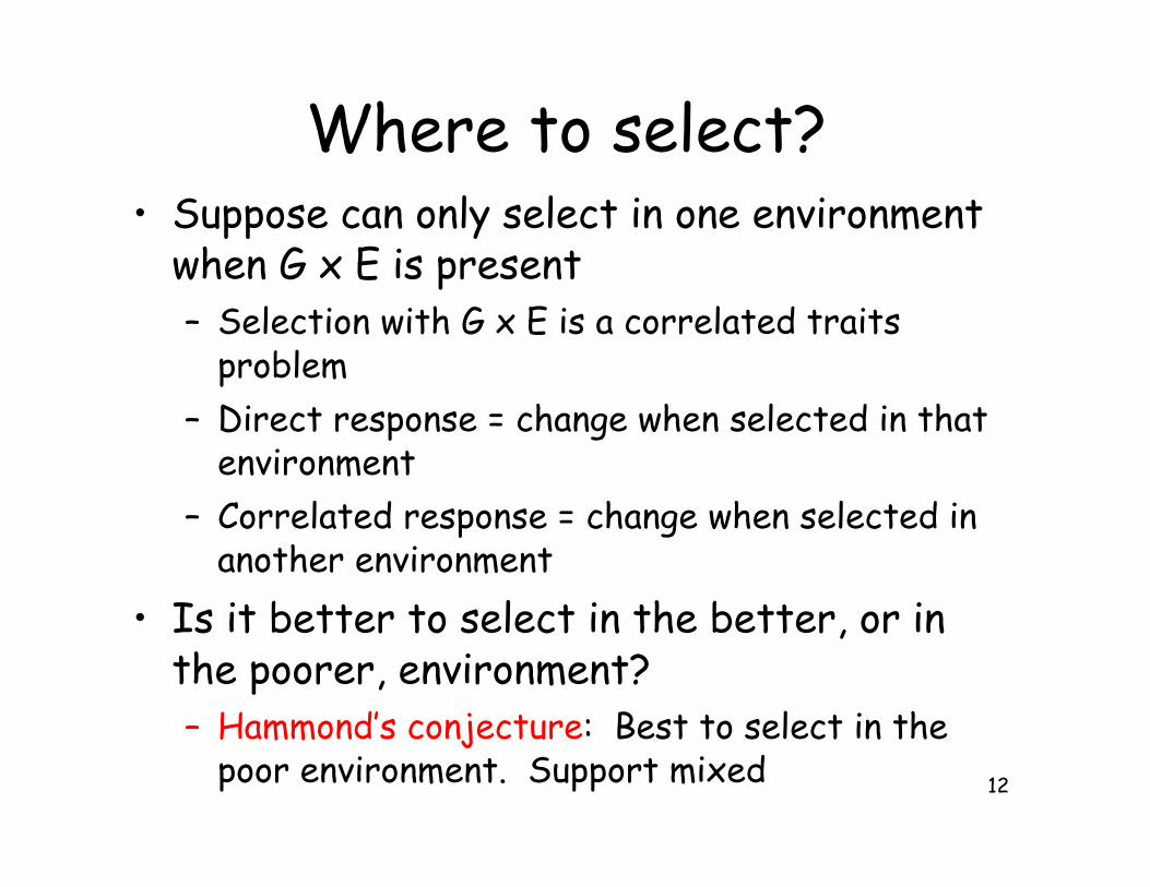
Where to select?• Suppose can only select in one environment
when G x E is present– Selection with G x E is a correlated traits
problem
– Direct response = change when selected in thatenvironment
– Correlated response = change when selected inanother environment
• Is it better to select in the better, or inthe poorer, environment?– Hammond’s conjecture: Best to select in the
poor environment. Support mixed
13
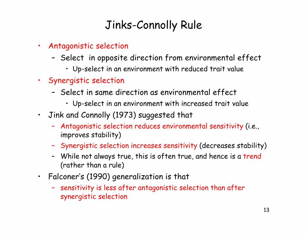
Jinks-Connolly Rule
• Antagonistic selection
– Select in opposite direction from environmental effect• Up-select in an environment with reduced trait value
• Synergistic selection
– Select in same direction as environmental effect
• Up-select in an environment with increased trait value
• Jink and Connolly (1973) suggested that– Antagonistic selection reduces environmental sensitivity (i.e.,
improves stability)
– Synergistic selection increases sensitivity (decreases stability)
– While not always true, this is often true, and hence is a trend(rather than a rule)
• Falconer’s (1990) generalization is that– sensitivity is less after antagonistic selection than after
synergistic selection

14
Estimating the GE term• While GE can be estimated directly from the mean in a cell
(i.e., Gi in Ej), we can usually get more information (and abetter estimate) by considering the entire design andexploiting structure in the GE terms
• This approach also allows us to potentially predict the GEterms in specific environments
• Basic idea: replace GEij by "i#j or more generally by $k "ki#kj
These are called biadditive or bilinear models. This (at firstsight) seems more complicated. Why do this?
• With nG genotypes and nE environments, we have
– nG nE GE terms (assuming no missing values)
– nG + nE "i and #i unique terms
– k(nG + nE) unique terms in $k "ki#kj .
• Suppose 50 genotypes in 10 environments– 500 GEij terms, 60 unique "i and #i terms, and (for k=3), 180
unique "ki and #ki terms.
15
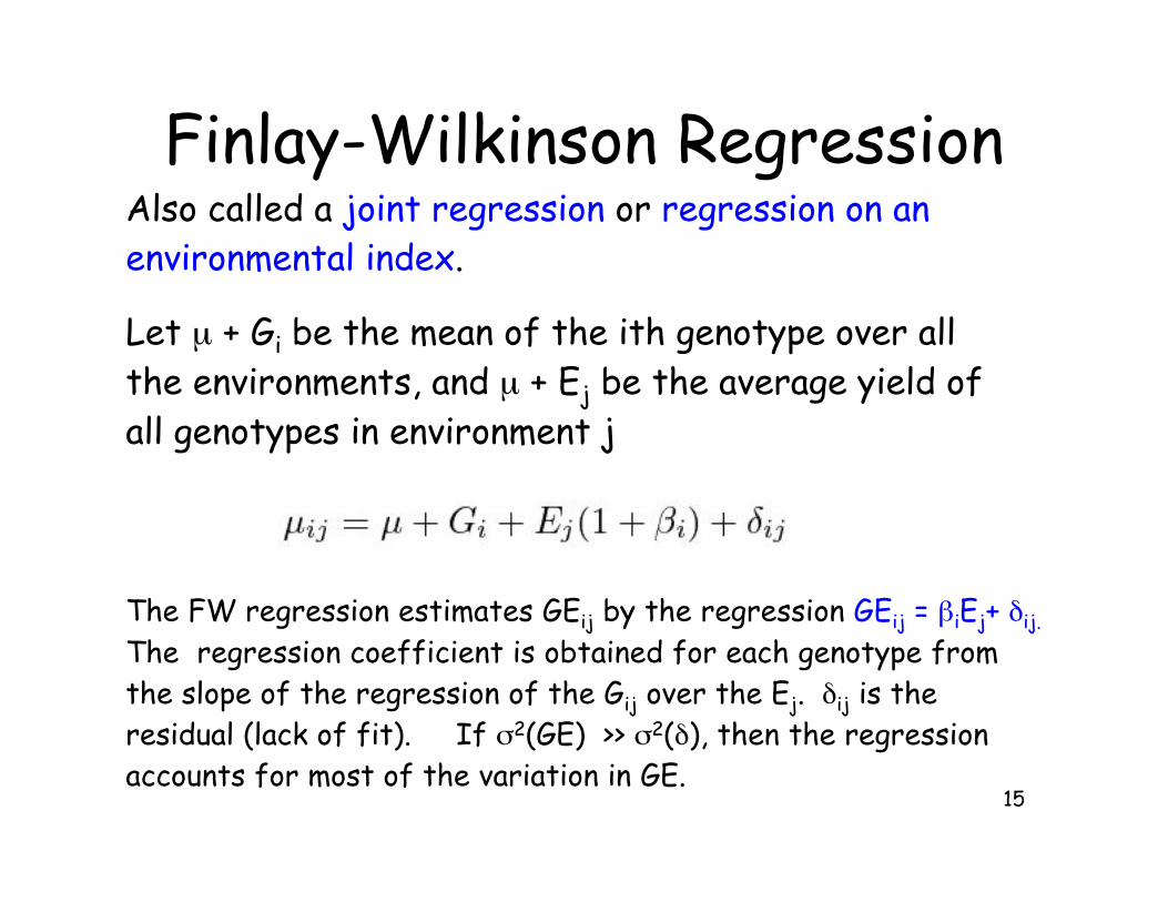
Finlay-Wilkinson RegressionAlso called a joint regression or regression on an environmental index.
Let µ + Gi be the mean of the ith genotype over allthe environments, and µ + Ej be the average yield ofall genotypes in environment j
The FW regression estimates GEij by the regression GEij = %iEj+ &ij.
The regression coefficient is obtained for each genotype fromthe slope of the regression of the Gij over the Ej. &ij is theresidual (lack of fit). If !2(GE) >> !2(&), then the regressionaccounts for most of the variation in GE.

16
Application• Yield in lines of wheat over different
environments was examined by Calderiniand Slafer (1999). The lines they examinedwhere lines from different eras ofbreeding (for four different countries)
• Newer lines had larger values, but also hadhigher slopes (large %i values), indicatingless stability over mean environmentalconditions than see in older lines

17Regression slope for each genotype is %i

18
% and Stability
• Since predicted GEij term is %iEj, %i measures the sensitivityof genotype i over the sampled environments
– Positive % implies sign of GE = sign of E
• Good environment = extra gain from positive GE
• Poorer environment = extra loss from negative GE
– Negative % implies sign of GE opposite of sign of E
• Performs better in poorer environments
– Large |%| implies a higher sensitivity over environments
– %i = -1 implies µ ij = µ + Gi + &ij (no dependence on Ej)
19
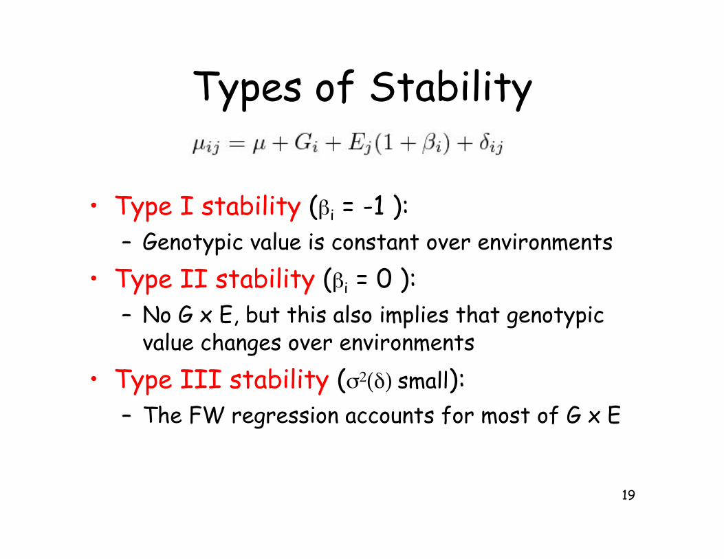
Types of Stability
• Type I stability (%i = -1 ):– Genotypic value is constant over environments
• Type II stability (%i = 0 ):– No G x E, but this also implies that genotypic
value changes over environments
• Type III stability (!2(&) small):– The FW regression accounts for most of G x E

20
SVD approaches• In Finlay-Wilkinson, the GEij term was estimated
by %iEj, where Ej was observed. We could alsohave used #jGi, where #j is the regression ofgenotype values over the j-th environment. AgainGi is observable.
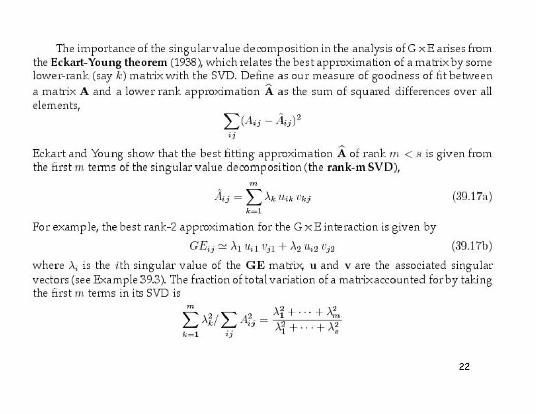
• Singular-value decomposition (SVD) approachesconsider a more general approach, approximatingGEij by $k "ki#kj where the "ki and #kj aredetermined by the first k terms in the SVD of thematrix of GE terms.
• The SVD is a way to obtain the best approximationof a full matrix by some matrix of lower dimension

21
22

23
A data set for soybeans grown in New York (Gauch 1992) gives theGE matrix as
Where GEij = value forGenotype i in envir. j

24
For example, the rank-1 SVD approximation for GE32 isg31'1e12 = 746.10*(-0.66)*0.64 = -315
While the rank-2 SVD approximation is g31'2e12 + g32'2e22 = 746.10*(-0.66)*0.64 + 131.36* 0.12*(-0.51) = -323
Actual value is -324
Generally, the rank-2 SVD approximation for GEij isgi1'1e1j + gi2'2e2j

25
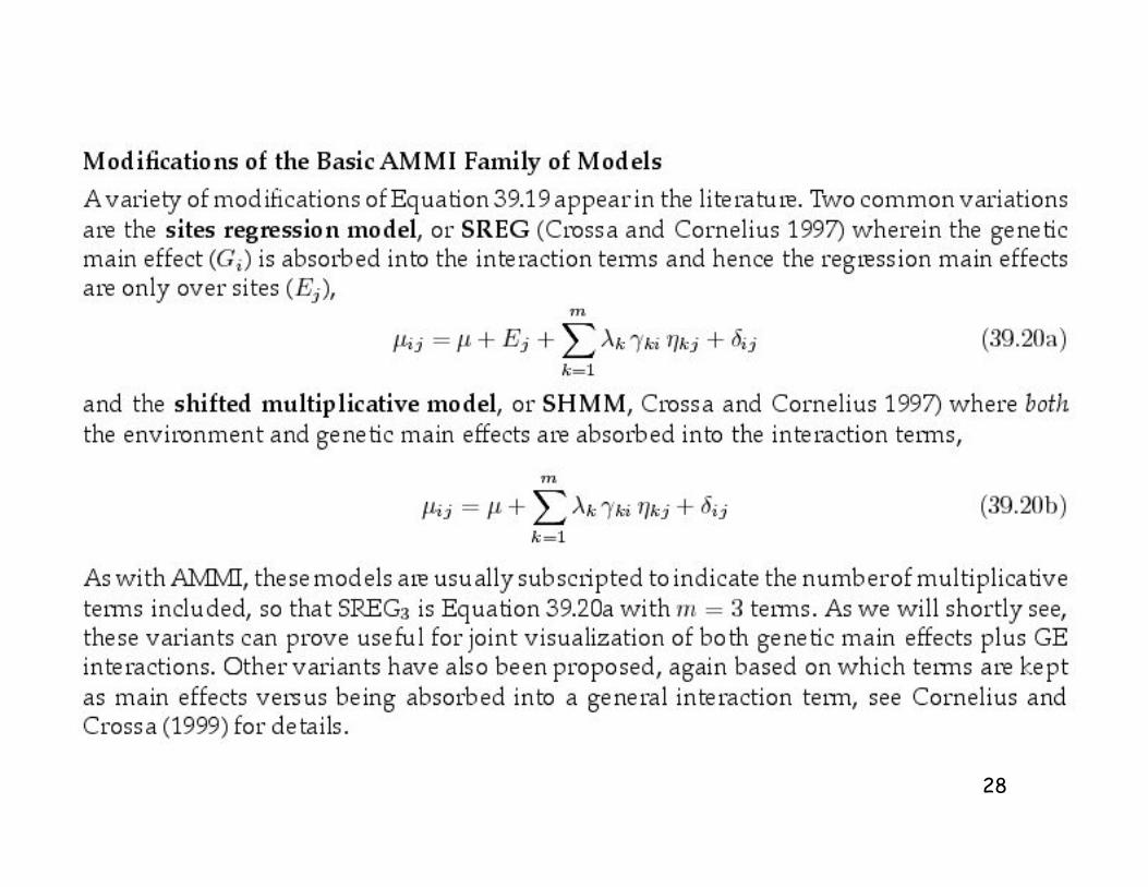
AMMI modelsAdditive main effects, multiplicative interaction (AMMI)models use the first m terms in the SVD of GE:
Giving
AMMI is actually a family of models, with AMMIm denoting AMMI with the first m SVD terms

26
AMMI models
Fit main effects
Fit principal componentsto the interaction term(SVD is a generalizationof PC methods)

27
Why do AMMI?• One can plot the SVD terms (#ki, (kj) to visualize
interactions
– Called biplots (see online notes Chapter 33 fordetails)
• AMMI can better estimate mean values of GEij
than just using the cell value (the observed mean
of Genotype i in Environment j)
• AMMI can predict GE values for genotype-environment combination not measured
• A huge amount more on AMMI in the online notes(Chapter 33)!
28

29
Factorial Regressions• While AMMI models attempt to extract information
about how G x E interactions are related across setsof genotypes and environments, factorial regressionsincorporate direct measures of environmentalfactors in an attempt to account for the observedpattern of G x E.
• The power of this approach is that if we candetermine which genotypes are more (or less)sensitive to which environmental features, thebreeder may be able to more finely tailor a line to aparticular environment without necessarily requiringtrials in the target environment.

30
Suppose we have a series of m measured values fromthe environments of interest (such as average rainfall,maximum temperature, etc.) Let xkj denote the value of the k-th environmental variable in environment j
Factorial regressions then model the GE term asthe sensitivity )ki of environmentalvalue k to genotype i, (this is a regression slope to be estimated from the data)
Note that the Finlay-Wilkinson regression is a specialcase where m = 1 and xj is the mean trait value (overall genotypes) in that environment.

31


