Page 1
Structured Matrix Computations from Structured Tensors
Lecture 1. Matrix-Tensor Connections
Charles F. Van Loan
Cornell University
CIME-EMS Summer SchoolJune 22-26, 2015
Cetraro, Italy
Structured Matrix Computations from Structured Tensors Lecture 1. Matrix-Tensor Connections 1 / 60
Page 2
Using examples, let us first takea look at what we might
mean by“hidden structure”
in a matrix.
Structured Matrix Computations from Structured Tensors Lecture 1. Matrix-Tensor Connections 2 / 60
Page 3
Hidden Matrix Structure: Five Motivating Examples
The Discrete Fourier Transform
Definition
F4 =
1 1 1 1
1 ω4 ω24 ω3
4
1 ω24 ω4
4 ω64
1 ω34 ω6
4 ω94
ωn = cos
(2π
n
)− i sin
(2π
n
)
Hidden Structure
F2mΠ2,m =
[Fm ΩmFm
Fm −ΩmFm
]Π2,m = perfect shuffle
Ωm = diagonal
Recursive Block StructureStructured Matrix Computations from Structured Tensors Lecture 1. Matrix-Tensor Connections 3 / 60
Page 4
Hidden Matrix Structure: Five Motivating Examples
The DFT Matrix is Data Sparse
The DFT matrix is dense, but can be factored into a product ofsparse matrices:
F1024 = A10 · · ·A2A1PT
The Ak have the form I ⊗[
I D
I −D
], D = diagonal.
That is what makes the FFT possible:
y = xfor k = 1:10
y = Aky
An N-by-N matrix is data sparse if it can be represented with manyfewer than N2 numbers. FN is data sparse: O(N log N) vs O(N2).
Structured Matrix Computations from Structured Tensors Lecture 1. Matrix-Tensor Connections 4 / 60
Page 5
Hidden Matrix Structure: Five Motivating Examples
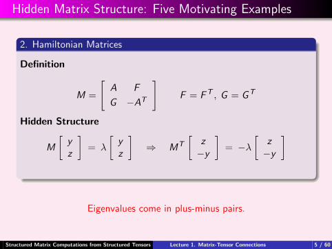
2. Hamiltonian Matrices
Definition
M =
[A F
G −AT
]F = FT , G = GT
Hidden Structure
M
[yz
]= λ
[yz
]⇒ MT
[z−y
]= −λ
[z−y
]
Eigenvalues come in plus-minus pairs.
Structured Matrix Computations from Structured Tensors Lecture 1. Matrix-Tensor Connections 5 / 60
Page 6
Hidden Matrix Structure: Five Motivating Examples
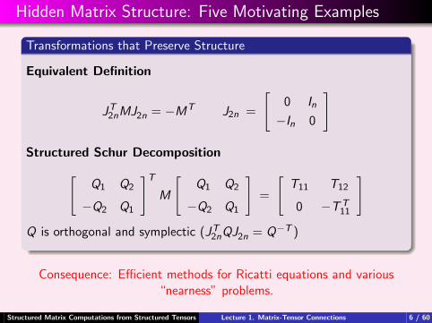
Transformations that Preserve Structure
Equivalent Definition
JT2nMJ2n = −MT J2n =
[0 In
−In 0
]
Structured Schur Decomposition[Q1 Q2
−Q2 Q1
]T
M
[Q1 Q2
−Q2 Q1
]=
[T11 T12
0 −TT11
]Q is orthogonal and symplectic (JT
2nQJ2n = Q−T )
Consequence: Efficient methods for Ricatti equations and various“nearness” problems.
Structured Matrix Computations from Structured Tensors Lecture 1. Matrix-Tensor Connections 6 / 60
Page 7
Hidden Matrix Structure: Five Motivating Examples
3. Cauchy Matrices
Definition
A = (akj) =
(1
ωk − λj
)=
1
ω1−λ1
1ω1−λ2
1ω1−λ3
1ω1−λ4
1ω2−λ1
1ω2−λ2
1ω2−λ3
1ω2−λ4
1ω3−λ1
1ω3−λ2
1ω3−λ3
1ω3−λ4
1ω4−λ1
1ω4−λ2
1ω4−λ3
1ω4−λ4
Hidden Structure
ΩA− AΛ = Rank-1 Ω = diag(ωi ), Λ = diag(λi ),
With respect to Ω and Λ, A has displacement rank equal to one.
Structured Matrix Computations from Structured Tensors Lecture 1. Matrix-Tensor Connections 7 / 60
Page 8
Hidden Matrix Structure: Five Motivating Examples
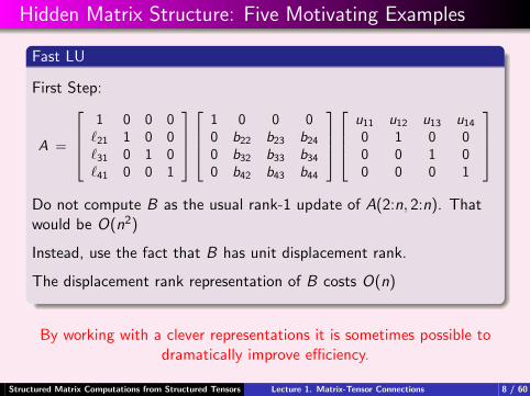
Fast LU
First Step:
A =
1 0 0 0
`21 1 0 0`31 0 1 0`41 0 0 1
1 0 0 00 b22 b23 b24
0 b32 b33 b34
0 b42 b43 b44
u11 u12 u13 u14
0 1 0 00 0 1 00 0 0 1
Do not compute B as the usual rank-1 update of A(2:n, 2:n). Thatwould be O(n2)
Instead, use the fact that B has unit displacement rank.
The displacement rank representation of B costs O(n)
By working with a clever representations it is sometimes possible todramatically improve efficiency.
Structured Matrix Computations from Structured Tensors Lecture 1. Matrix-Tensor Connections 8 / 60
Page 9
Hidden Matrix Structure: Five Motivating Examples
4. Matrices with Orthonormal Columns
Definition
Q =
[Q1
Q2
]QT
1 Q1 + QT2 Q2 = I
Hidden Structure[U1 0
0 U2
]T [Q1
Q2
]V =
[diag(ci )
diag(si )
]c2i + s2
i = 1
U1, U2, V = orthogonal
Q1 and Q2 have related SVDs. This is the CS Decomposition.
Structured Matrix Computations from Structured Tensors Lecture 1. Matrix-Tensor Connections 9 / 60
Page 10
Hidden Matrix Structure: Five Motivating Examples
Simultaneous Diagonalization of A1 and A2
1. QR factorization:
[A1
A2
]=
[Q1
Q2
]R
2. CS decomposition:
[U1 0
0 U2
]T [Q1
Q2
]V =
[diag(ci )
diag(si )
]c2i + s2
i = 1
3. Setting X = RTV gives the generalized singularvalue decomposition:
A1 = U1 ·diag(ci )·XT A2 = U2 ·diag(si )·XT
An example where exploiting the hidden structure of Q1 and Q2
ensures numerical stability.
Structured Matrix Computations from Structured Tensors Lecture 1. Matrix-Tensor Connections 10 / 60
Page 11
Hidden Matrix Structure: Five Motivating Examples
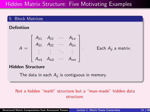
5. Block Matrices
Definition
A =
A11 A12 · · · A1N
A21 A22 · · · A2N
......
. . ....
AM1 AM2 · · · AMN
. Each Aij a matrix.
Hidden Structure
The data in each Aij is contiguous in memory.
Not a hidden “math” structure but a “man-made” hidden datastructure.
Structured Matrix Computations from Structured Tensors Lecture 1. Matrix-Tensor Connections 11 / 60
Page 12
Hidden Matrix Structure: Five Motivating Examples
Respect Data Layout to Minimize Memory Traffic
A ←
AT
11 AT12 · · · AT
1N
AT21 AT
22 · · · AT2N
......
. . ....
ATM1 AT
M2 · · · ATMN
. Overwrite Aij with ATij .
A ←
AT
11 AT21 · · · AT
M1
AT12 AT
22 · · · ATM2
......
. . ....
AT1N
AT2N· · · AT
MN
. Swap ATij with AT
ji
A 2-pass transpose that exploits the “hidden” data structure.
Structured Matrix Computations from Structured Tensors Lecture 1. Matrix-Tensor Connections 12 / 60
Page 13
Hidden Structure in Matrices
Each of these examples has a connection to our agenda:
MondayLecture 1. Matrix-tensor Connections
Lecture 2. Tensor Symmetries and RankTuesday
Lecture 3. The Tucker and Tensor Train Representations
Lecture 4. The CP and KSVD RepresentationsThursday
Lecture 5. Unfolding a Tensor with Multiple Symmetries
Lecture 6. A Higher-Order GSVD
Structured Matrix Computations from Structured Tensors Lecture 1. Matrix-Tensor Connections 13 / 60
Page 14
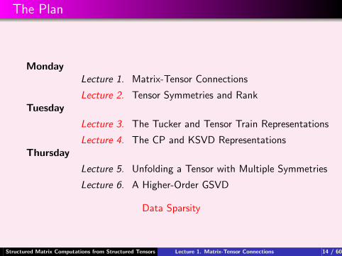
The Plan
MondayLecture 1. Matrix-Tensor Connections
Lecture 2. Tensor Symmetries and RankTuesday
Lecture 3. The Tucker and Tensor Train Representations
Lecture 4. The CP and KSVD RepresentationsThursday
Lecture 5. Unfolding a Tensor with Multiple Symmetries
Lecture 6. A Higher-Order GSVD
Data Sparsity
Structured Matrix Computations from Structured Tensors Lecture 1. Matrix-Tensor Connections 14 / 60
Page 15
The Plan
MondayLecture 1. Matrix-Tensor Connections
Lecture 2. Tensor Symmetries and RankTuesday
Lecture 3. The Tucker and Tensor Train Representations
Lecture 4. The CP and KSVD RepresentationsThursday
Lecture 5. Unfolding a Tensor with Multiple Symmetries
Lecture 6. A Higher-Order GSVD
Structured Permutation Similarity
Structured Matrix Computations from Structured Tensors Lecture 1. Matrix-Tensor Connections 15 / 60
Page 16
The Plan
MondayLecture 1. Matrix-Tensor Connections
Lecture 2. Tensor Symmetries and RankTuesday
Lecture 3. The Tucker and Tensor Train Representations
Lecture 4. The CP and KSVD RepresentationsThursday
Lecture 5. Unfolding a Tensor with Multiple Symmetries
Lecture 6. A Higher-Order GSVD
A Higher-Order CS Decompositions
Structured Matrix Computations from Structured Tensors Lecture 1. Matrix-Tensor Connections 16 / 60
Page 17
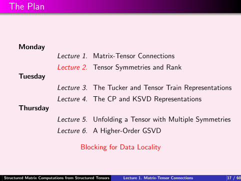
The Plan
MondayLecture 1. Matrix-Tensor Connections
Lecture 2. Tensor Symmetries and RankTuesday
Lecture 3. The Tucker and Tensor Train Representations
Lecture 4. The CP and KSVD RepresentationsThursday
Lecture 5. Unfolding a Tensor with Multiple Symmetries
Lecture 6. A Higher-Order GSVD
Blocking for Data Locality
Structured Matrix Computations from Structured Tensors Lecture 1. Matrix-Tensor Connections 17 / 60
Page 18
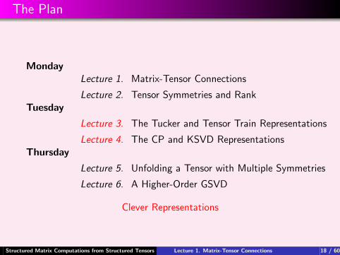
The Plan
MondayLecture 1. Matrix-Tensor Connections
Lecture 2. Tensor Symmetries and RankTuesday
Lecture 3. The Tucker and Tensor Train Representations
Lecture 4. The CP and KSVD RepresentationsThursday
Lecture 5. Unfolding a Tensor with Multiple Symmetries
Lecture 6. A Higher-Order GSVD
Clever Representations
Structured Matrix Computations from Structured Tensors Lecture 1. Matrix-Tensor Connections 18 / 60
Page 19
Let us Begin!
Structured Matrix Computations from Structured Tensors Lecture 1. Matrix-Tensor Connections 19 / 60
Page 20
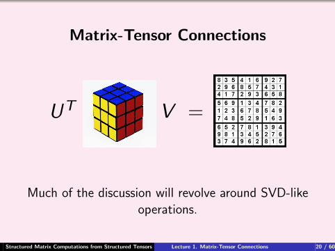
Matrix-Tensor Connections
UT V =
Much of the discussion will revolve around SVD-likeoperations.
Structured Matrix Computations from Structured Tensors Lecture 1. Matrix-Tensor Connections 20 / 60
Page 21
What is a Tensor?
Structured Matrix Computations from Structured Tensors Lecture 1. Matrix-Tensor Connections 21 / 60
Page 22
What is a Tensor?
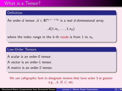
Definition
An order-d tensor A ∈ IRn1×···×nd is a real d-dimensional array
A(1:n1, . . . , 1:nd)
where the index range in the k-th mode is from 1 to nk .
Low-Order Tensors
A scalar is an order-0 tensor.
A vector is an order-1 tensor.
A matrix is an order-2 tensor.
We use calligraphic font to designate tensors that have order 3 or greatere.g., A, B, C, etc.
Structured Matrix Computations from Structured Tensors Lecture 1. Matrix-Tensor Connections 22 / 60
Page 23
Parts of a Tensor
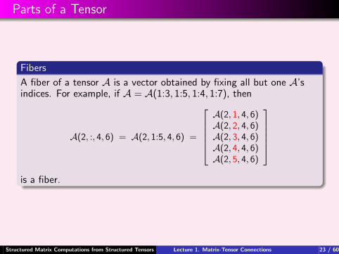
Fibers
A fiber of a tensor A is a vector obtained by fixing all but one A’sindices. For example, if A = A(1:3, 1:5, 1:4, 1:7), then
A(2, :, 4, 6) = A(2, 1:5, 4, 6) =
A(2, 1, 4, 6)A(2, 2, 4, 6)A(2, 3, 4, 6)A(2, 4, 4, 6)A(2, 5, 4, 6)
is a fiber.
Structured Matrix Computations from Structured Tensors Lecture 1. Matrix-Tensor Connections 23 / 60
Page 24
Parts of a Tensor
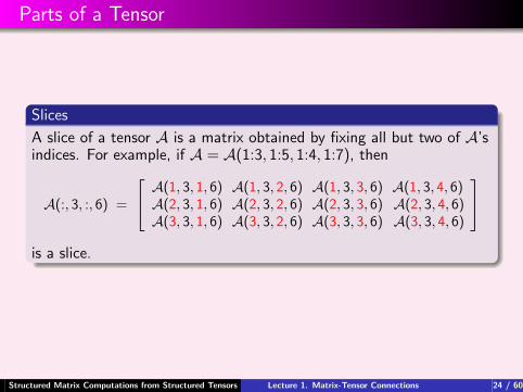
Slices
A slice of a tensor A is a matrix obtained by fixing all but two of A’sindices. For example, if A = A(1:3, 1:5, 1:4, 1:7), then
A(:, 3, :, 6) =
A(1, 3, 1, 6) A(1, 3, 2, 6) A(1, 3, 3, 6) A(1, 3, 4, 6)A(2, 3, 1, 6) A(2, 3, 2, 6) A(2, 3, 3, 6) A(2, 3, 4, 6)A(3, 3, 1, 6) A(3, 3, 2, 6) A(3, 3, 3, 6) A(3, 3, 4, 6)
is a slice.
Structured Matrix Computations from Structured Tensors Lecture 1. Matrix-Tensor Connections 24 / 60
Page 25
Where Might They Come From?
Discretization
A(i , j , k, `) might house the value of f (w , x , y , z) at(w , x , y , z) = (wi , xj , yk , z`).
Multiway Analysis
A(i , j , k, `) is a value that captures an interaction between fourvariables/factors.
Structured Matrix Computations from Structured Tensors Lecture 1. Matrix-Tensor Connections 25 / 60
Page 26
You Have Seen them Before
Block Matrices (With Uniformly-Sized Blocks)
A =
a11 a12 a13 a14 a15 a16
a21 a22 a23 a24 a25 a26
a31 a32 a33 a34 a35 a36
a41 a42 a43 a44 a45 a46
a51 a52 a53 a54 a55 a56
a61 a62 a63 a64 a65 a66
Matrix entry a45 is the (2,1) entry of the (2,3) block:
a45 ⇔ A(2, 3, 2, 1)
Structured Matrix Computations from Structured Tensors Lecture 1. Matrix-Tensor Connections 26 / 60
Page 27
You Have Seen Them Before
Kronecker Products (At the Scalar Level)
A =
b11 b12 b13
b21 b22 b23
b31 b32 b33
⊗ [c11 c12
c21 c22
]
=
b11c11 b11c12 b12c11 b12c12 b13c11 b13c12
b11c21 b11c22 b12c21 b12c22 b13c21 b13c22
b21c11 b21c12 b22c11 b22c12 b23c11 b23c12
b21c21 b21c22 b22c21 b22c22 b23c21 b23c22
b31c11 b31c12 b32c11 b32c12 b33c11 b33c12
b31c21 b31c22 b32c21 b32c22 b33c21 b33c22
Matrix A is an unfolding of tensor A where A(p, q, r , s) = bpqcrs .
Structured Matrix Computations from Structured Tensors Lecture 1. Matrix-Tensor Connections 27 / 60
Page 28
You Have Seen Them Before
Kronecker Products (At the Block Level)
A =
b11 b12 b13
b21 b22 b23
b31 b32 b33
⊗ [c11 c12
c21 c22
]
=
b11C b12C b13C
b21C b22C b23C
b31C b32C b33C
Matrix A is a block matrix whose ij block is bijC .
Structured Matrix Computations from Structured Tensors Lecture 1. Matrix-Tensor Connections 28 / 60
Page 29
You Have Seen Them Before
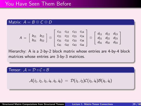
Matrix: A = B ⊗ C ⊗ D
A =
[b11 b12
b21 b22
]⊗
c11 c12 c13 c14
c21 c22 c23 c24
c31 c32 c33 c34
c41 c42 c43 c44
⊗ d11 d12 d13
d21 d22 d23
d31 d32 d33
Hierarchy: A is a 2-by-2 block matrix whose entries are 4-by-4 blockmatrices whose entries are 3-by-3 matrices.
Tensor: A = D C B
A(i1, i2, i3, i4, i5, i6) = D(i1, i2)C(i3, i4)B(i5, i6)
Structured Matrix Computations from Structured Tensors Lecture 1. Matrix-Tensor Connections 29 / 60
Page 30
A First Look at Tensor Symmetry
Let’s look at the connection betweenKronecker products and tensors
when symmetry is present.
Structured Matrix Computations from Structured Tensors Lecture 1. Matrix-Tensor Connections 30 / 60
Page 31
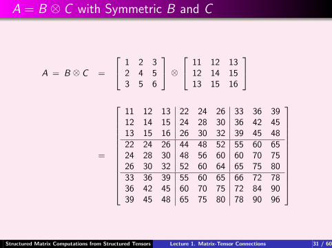
A = B ⊗ C with Symmetric B and C
A = B ⊗ C =
1 2 32 4 53 5 6
⊗ 11 12 13
12 14 1513 15 16
=
11 12 13 22 24 26 33 36 3912 14 15 24 28 30 36 42 4513 15 16 26 30 32 39 45 4822 24 26 44 48 52 55 60 6524 28 30 48 56 60 60 70 7526 30 32 52 60 64 65 75 8033 36 39 55 60 65 66 72 7836 42 45 60 70 75 72 84 9039 45 48 65 75 80 78 90 96
Structured Matrix Computations from Structured Tensors Lecture 1. Matrix-Tensor Connections 31 / 60
Page 32
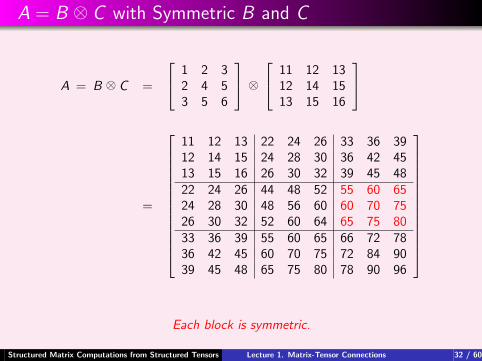
A = B ⊗ C with Symmetric B and C
A = B ⊗ C =
1 2 32 4 53 5 6
⊗ 11 12 13
12 14 1513 15 16
=
11 12 13 22 24 26 33 36 3912 14 15 24 28 30 36 42 4513 15 16 26 30 32 39 45 4822 24 26 44 48 52 55 60 6524 28 30 48 56 60 60 70 7526 30 32 52 60 64 65 75 8033 36 39 55 60 65 66 72 7836 42 45 60 70 75 72 84 9039 45 48 65 75 80 78 90 96
Each block is symmetric.
Structured Matrix Computations from Structured Tensors Lecture 1. Matrix-Tensor Connections 32 / 60
Page 33
A = B ⊗ C with Symmetric B and C
A = B ⊗ C =
1 2 32 4 53 5 6
⊗ 11 12 13
12 14 1513 15 16
=
11 12 13 22 24 26 33 36 3912 14 15 24 28 30 36 42 4513 15 16 26 30 32 39 45 4822 24 26 44 48 52 55 60 6524 28 30 48 56 60 60 70 7526 30 32 52 60 64 65 75 8033 36 39 55 60 65 66 72 7836 42 45 60 70 75 72 84 9039 45 48 65 75 80 78 90 96
Block (i , j) equals Block (j , i)
Structured Matrix Computations from Structured Tensors Lecture 1. Matrix-Tensor Connections 33 / 60
Page 34
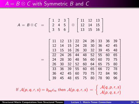
A = B ⊗ C with Symmetric B and C
A = B ⊗ C =
1 2 32 4 53 5 6
⊗ 11 12 13
12 14 1513 15 16
=
11 12 13 22 24 26 33 36 3912 14 15 24 28 30 36 42 4513 15 16 26 30 32 39 45 4822 24 26 44 48 52 55 60 6524 28 30 48 56 60 60 70 7526 30 32 52 60 64 65 75 8033 36 39 55 60 65 66 72 7836 42 45 60 70 75 72 84 9039 45 48 65 75 80 78 90 96
If A(p, q, r , s) = bpqcrs then A(p, q, r , s) =
A(q, p, r , s)A(p, q, s, r)
Structured Matrix Computations from Structured Tensors Lecture 1. Matrix-Tensor Connections 34 / 60
Page 35
A = B ⊗ B with Symmetric B
A = B ⊗ B =
4 5 65 7 86 8 9
⊗ 4 5 6
5 7 86 8 9
=
16 20 24 20 25 30 24 30 36
20 28 32 25 35 40 30 42 4824 32 36 30 40 45 36 48 5420 25 30 28 35 42 32 40 48
25 35 40 35 49 56 40 56 6430 40 45 42 56 63 48 64 7224 30 36 32 40 48 36 45 54
30 42 48 40 56 64 45 63 7236 48 54 48 64 72 54 72 81
Block(i , j) = A(i :n:n2, j :n:n2) Block(2, 3) = A(2:3:9, 3:3:9)
Structured Matrix Computations from Structured Tensors Lecture 1. Matrix-Tensor Connections 35 / 60
Page 36
A = B ⊗ B with Symmetric B
A = B ⊗ B =
4 5 65 7 86 8 9
⊗ 4 5 6
5 7 86 8 9
=
16 20 24 20 25 30 24 30 3620 28 32 25 35 40 30 42 4824 32 36 30 40 45 36 48 5420 25 30 28 35 42 32 40 4825 35 40 35 49 56 40 56 6430 40 45 42 56 63 48 64 7224 30 36 32 40 48 36 45 5430 42 48 40 56 64 45 63 7236 48 54 48 64 72 54 72 81
If A(p, q, r , s) = bpqbrs then A(p, q, r , s) =
A(q, p, r , s)A(p, q, s, r)A(r , s, p, q)
Structured Matrix Computations from Structured Tensors Lecture 1. Matrix-Tensor Connections 36 / 60
Page 37
A First Look at Tensor Symmetry
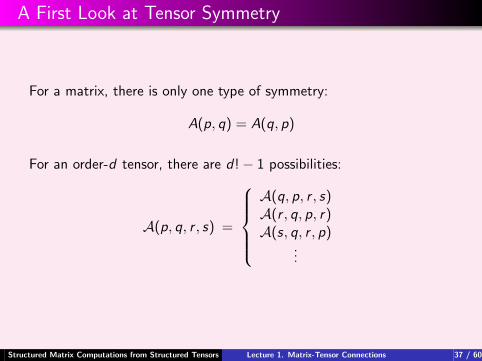
For a matrix, there is only one type of symmetry:
A(p, q) = A(q, p)
For an order-d tensor, there are d!− 1 possibilities:
A(p, q, r , s) =
A(q, p, r , s)A(r , q, p, r)A(s, q, r , p)
...
Structured Matrix Computations from Structured Tensors Lecture 1. Matrix-Tensor Connections 37 / 60
Page 38
A First Look at Rank-1 Tensors
Next, let’s look at the connection betweenKronecker products and tensors
in the rank-1 setting.
Structured Matrix Computations from Structured Tensors Lecture 1. Matrix-Tensor Connections 38 / 60
Page 39
Rank-1 Reshaping
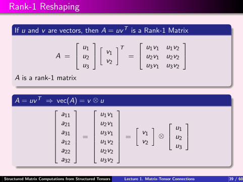
If u and v are vectors, then A = uvT is a Rank-1 Matrix
A =
u1
u2
u3
[v1
v2
]T
=
u1v1 u1v2
u2v1 u2v2
u3v1 u3v2
A is a rank-1 matrix
A = uvT ⇒ vec(A) = v ⊗ u
a11
a21
a31
a12
a22
a32
=
u1v1
u2v1
u3v1
u1v2
u2v2
u3v2
=
[v1
v2
]⊗
u1
u2
u3
Structured Matrix Computations from Structured Tensors Lecture 1. Matrix-Tensor Connections 39 / 60
Page 40
In the Language of Tensor Products
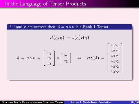
If u and v are vectors then A = u v is a Rank-1 Tensor
A(i1, i2) = u(i1)v(i2)
A = u v =
u1
u2
u3
[v1
v2
]⇔ vec(A) =
u1v1
u2v1
u3v1
u1v2
u2v2
u3v2
Structured Matrix Computations from Structured Tensors Lecture 1. Matrix-Tensor Connections 40 / 60
Page 41
Higher-Order Rank-1 Tensors
If u, v , and w are vectors, then A = u v w is a Rank-1 Tensor
A(p, q, r) = upvqwr
A = uvw =
[u1
u2
][
v1
v2
][
w1
w2
]⇒ vec(A) =
u1v1w1
u2v1w1
u1v2w1
u2v2w1
u1v1w2
u2v1w2
u1v2w2
u2v2w2
A tensor product of d vectors produces an order-d rank-1 tensor.
Structured Matrix Computations from Structured Tensors Lecture 1. Matrix-Tensor Connections 41 / 60
Page 42
A Notation Detail: u-v-w versus w-v-u
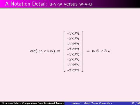
vec(u v w) ≡
u1v1w1
u2v1w1
u1v2w1
u2v2w1
u1v1w2
u2v1w2
u1v2w2
u2v2w2
= w ⊗ v ⊗ u
Structured Matrix Computations from Structured Tensors Lecture 1. Matrix-Tensor Connections 42 / 60
Page 43
A First Look at Multilinear Optimization
Let’s look at how we might compute thethe nearest rank-1 tensor to
a given tensor.
Structured Matrix Computations from Structured Tensors Lecture 1. Matrix-Tensor Connections 43 / 60
Page 44
The Nearest Rank-1 Problem for Matrices
Formulation:
Given A ∈ IRm×n, find unit-2 norm vectors u ∈ IRm and v ∈ IRn and anonnegative scalar σ that minimizes
φ(σ, u, v) = ‖ A− σuvT ‖F .
SVD Solution:
If UTAV = Σ = diag(σi ) where
U = [u1 | · · · | um] V = [v1 | · · · | vn]
are orthogonal and σ1 ≥ · · · ≥ σn ≥ 0, then σoptuoptvTopt = σ1u1v
T1 .
Structured Matrix Computations from Structured Tensors Lecture 1. Matrix-Tensor Connections 44 / 60
Page 45
The Nearest Rank-1 Problem for Matrices
An Alternating Least Squares Approach
v = unit vector
Repeat Until Happy:
% Fix v and choose σ and u to minimize ‖ A− σuvT ‖Fx = Av ; σ = ‖ x ‖; u = x/σ
% Fix u and choose σ and v to minimize ‖ A− σuvT ‖Fx = ATu; σ = ‖ x ‖; v = x/σ
σopt = σ; uopt = u; vopt = v
‖ A− σuvT ‖2F = trace(ATA)− 2σuTAv + σ2
The best u is in the direction of Av. The best v is in the direction of ATu.
Structured Matrix Computations from Structured Tensors Lecture 1. Matrix-Tensor Connections 45 / 60
Page 46
The Nearest Rank-1 Problem for Matrices
An Alternating Least Squares Approach
v = unit vector
Repeat Until Happy:
% Fix v and choose σ and u to minimize ‖ A− σuvT ‖Fx = Av ; σ = ‖ x ‖; u = x/σ
% Fix u and choose σ and v to minimize ‖ A− σuvT ‖Fx = ATu; σ = ‖ x ‖; v = x/σ
σopt = σ; uopt = u; vopt = v
This is just the power method applied to ATA:
x = (ATA)v , v = x/‖ x ‖
Structured Matrix Computations from Structured Tensors Lecture 1. Matrix-Tensor Connections 46 / 60
Page 47
Nearest Rank-1 Problem for Tensors
Formulation
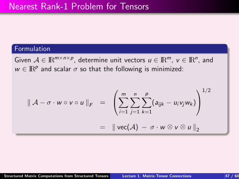
Given A ∈ IRm×n×p, determine unit vectors u ∈ IRm, v ∈ IRn, andw ∈ IRp and scalar σ so that the following is minimized:
‖ A − σ · w v u ‖F =
m∑i=1
n∑j=1
p∑k=1
(aijk − uivjwk)
1/2
= ‖ vec(A) − σ · w ⊗ v ⊗ u ‖2
Structured Matrix Computations from Structured Tensors Lecture 1. Matrix-Tensor Connections 47 / 60
Page 48
Nearest Rank-1 Problem for Tensors
Alternating Least Squares Framework for min‖ vec(A) − σ · w ⊗ v ⊗ u ‖2
v and w given unit vectors
Repeat Until Happy
Determine x ∈ IRm that minimizes ‖ vec(A) − w ⊗ v ⊗ x ‖2and set σ = ‖ x ‖ and u = x/σ
Determine y ∈ IRn that minimizes ‖ vec(A) − w ⊗ y ⊗ u ‖2and set σ = ‖ y ‖ and v = y/σ
Determine z ∈ IRp that minimizes ‖ vec(A) − z ⊗ v ⊗ u ‖2and set σ = ‖ z ‖ and w = z/σ
Details in next Lecture. For now, we look at the special structure ofthese linear least square problems for the case m = n = p = 2.
Structured Matrix Computations from Structured Tensors Lecture 1. Matrix-Tensor Connections 48 / 60
Page 49
The Nearest Rank-1 Problem for Tensors
The Case m = n = p = 2
minimize
∥∥∥∥∥∥∥∥∥∥∥∥∥∥∥∥
a111
a211
a121
a221
a112
a212
a122
a222
− σ · w ⊗ v ⊗ u
∥∥∥∥∥∥∥∥∥∥∥∥∥∥∥∥2
u =
»cos(θ1)sin(θ1)
–=
»c1
s1
–v =
»cos(θ2)sin(θ2)
–=
»c2
s2
–w =
»cos(θ3)sin(θ3)
–=
»c3
s3
–
Structured Matrix Computations from Structured Tensors Lecture 1. Matrix-Tensor Connections 49 / 60
Page 50
A Highly Structured Nonlinear Optimization Problem
It Depends on Four Parameters...
φ(σ, θ1, θ2, θ3) =
∥∥∥∥a − σ
[cos(θ3)sin(θ3)
]⊗
[cos(θ2)sin(θ2)
]⊗
[cos(θ1)sin(θ1)
]∥∥∥∥2
=
∥∥∥∥∥∥∥∥∥∥∥∥∥∥∥∥
a111
a211
a121
a221
a112
a212
a122
a222
− σ ·
c3c2c1
c3c2s1c3s2c1
c3s2s1s3c2c1
s3c2s1s3s2c1
s3s2s1
∥∥∥∥∥∥∥∥∥∥∥∥∥∥∥∥2
Structured Matrix Computations from Structured Tensors Lecture 1. Matrix-Tensor Connections 50 / 60
Page 51
A Highly Structured Nonlinear Optimization Problem
Set x1 = σ cos(θ1) and y1 = σ sin(θ1) and then Reshape...
φ =
‚‚‚‚‚‚‚‚‚‚‚‚‚‚‚‚
266666666664
a111
a211
a121
a221
a112
a212
a122
a222
377777777775− σ ·
266666666664
c3c2c1
c3c2s1
c3s2c1
c3s2s1
s3c2c1
s3c2s1
s3s2c1
s3s2s1
377777777775
‚‚‚‚‚‚‚‚‚‚‚‚‚‚‚‚2
=
‚‚‚‚‚‚‚‚‚‚‚‚‚‚‚‚
266666666664
a111
a211
a121
a221
a112
a212
a122
a222
377777777775−
266666666664
c3c2 00 c3c2
c3s2 00 c3s2
s3c2 00 s3c2
s3s2 00 s3s2
377777777775
»x1
y1
– ‚‚‚‚‚‚‚‚‚‚‚‚‚‚‚‚2
This is an ordinary linear least squares problem for x1 and y1 if we ”freeze”θ2 and θ3. Solve and update σ and u1 using[
x1
y1
]= σu1 σ =
√x21 + y2
1
Structured Matrix Computations from Structured Tensors Lecture 1. Matrix-Tensor Connections 51 / 60
Page 52
A Highly Structured Nonlinear Optimization Problem
Set x2 = σ cos(θ2) and y2 = σ sin(θ2) and then Reshape...
φ =
‚‚‚‚‚‚‚‚‚‚‚‚‚‚‚‚
266666666664
a111
a211
a121
a221
a112
a212
a122
a222
377777777775− σ ·
266666666664
c3c2c1
c3c2s1
c3s2c1
c3s2s1
s3c2c1
s3c2s1
s3s2c1
s3s2s1
377777777775
‚‚‚‚‚‚‚‚‚‚‚‚‚‚‚‚2
=
‚‚‚‚‚‚‚‚‚‚‚‚‚‚‚‚
266666666664
a111
a211
a121
a221
a112
a212
a122
a222
377777777775−
266666666664
c3c1 0c3s1 00 c3c1
0 c3s1
s3c1 0s3s1 00 s3c1
0 s3s1
377777777775
»x2
y2
– ‚‚‚‚‚‚‚‚‚‚‚‚‚‚‚‚2
This is an ordinary linear least squares problem for x2 and y2 if we ”freeze”θ1 and θ3. Solve and update σ and u2 using[
x2
y2
]= σu2 σ =
√x22 + y2
2
Structured Matrix Computations from Structured Tensors Lecture 1. Matrix-Tensor Connections 52 / 60
Page 53
A Highly Structured Nonlinear Optimization Problem
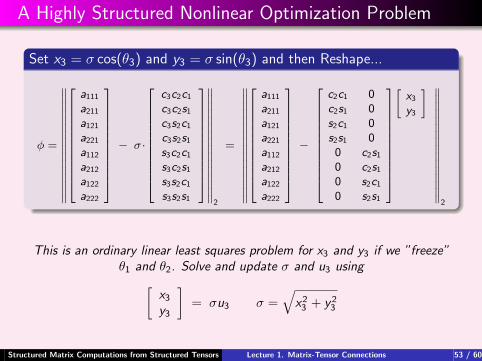
Set x3 = σ cos(θ3) and y3 = σ sin(θ3) and then Reshape...
φ =
‚‚‚‚‚‚‚‚‚‚‚‚‚‚‚‚
266666666664
a111
a211
a121
a221
a112
a212
a122
a222
377777777775− σ ·
266666666664
c3c2c1
c3c2s1
c3s2c1
c3s2s1
s3c2c1
s3c2s1
s3s2c1
s3s2s1
377777777775
‚‚‚‚‚‚‚‚‚‚‚‚‚‚‚‚2
=
‚‚‚‚‚‚‚‚‚‚‚‚‚‚‚‚
266666666664
a111
a211
a121
a221
a112
a212
a122
a222
377777777775−
266666666664
c2c1 0c2s1 0s2c1 0s2s1 00 c2s1
0 c2s1
0 s2c1
0 s2s1
377777777775
»x3
y3
– ‚‚‚‚‚‚‚‚‚‚‚‚‚‚‚‚2
This is an ordinary linear least squares problem for x3 and y3 if we ”freeze”θ1 and θ2. Solve and update σ and u3 using[
x3
y3
]= σu3 σ =
√x23 + y2
3
Structured Matrix Computations from Structured Tensors Lecture 1. Matrix-Tensor Connections 53 / 60
Page 54
Componentwise Optimization
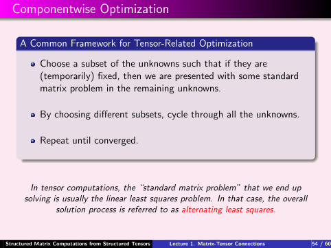
A Common Framework for Tensor-Related Optimization
Choose a subset of the unknowns such that if they are(temporarily) fixed, then we are presented with some standardmatrix problem in the remaining unknowns.
By choosing different subsets, cycle through all the unknowns.
Repeat until converged.
In tensor computations, the “standard matrix problem” that we end upsolving is usually the linear least squares problem. In that case, the overall
solution process is referred to as alternating least squares.
Structured Matrix Computations from Structured Tensors Lecture 1. Matrix-Tensor Connections 54 / 60
Page 55
Optional “Fun” Problems
Problem E1. Consider the the three linear least (LS) squares problemsthat arise when the alternating least squares framework is applied to the2-by-2-by-2 problem. Outline a solution approach when these linear LSproblems are solved using the method of normal equations. (Recall that themethod of normal equations for the LS problem min ‖Mu − b ‖2 involvessolving the symmetric positive definite linear system MTMu = MTb.)
Problem A1. Repeat E1 but when A ∈ IR2×2×···×2 is an order-d tensor.
Structured Matrix Computations from Structured Tensors Lecture 1. Matrix-Tensor Connections 55 / 60
Page 56
Closing Remarks
Structured Matrix Computations from Structured Tensors Lecture 1. Matrix-Tensor Connections 56 / 60
Page 57
Where Do We Go From Here?
To sums of rank-1’s...
vec(A) =r∑
k=1
σkwk ⊗ vk ⊗ uk
To more general unfoldings...
A ∈ IR4×2×3 ⇒
a111 a121 a131 a112 a122 a132
a211 a221 a231 a212 a222 a232
a311 a321 a331 a312 a322 a332
a411 a421 a431 a412 a422 a432
To more complicated multilinear optimizations...
minU, V , W ∈ IRn×n orthogonal
s ∈ IRn3
‖vec(A) − (W ⊗ V ⊗ U)s‖2
Structured Matrix Computations from Structured Tensors Lecture 1. Matrix-Tensor Connections 57 / 60
Page 58
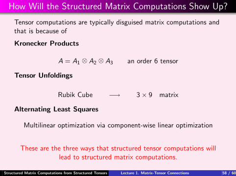
How Will the Structured Matrix Computations Show Up?
Tensor computations are typically disguised matrix computations andthat is because of
Kronecker Products
A = A1 ⊗ A2 ⊗ A3 an order 6 tensor
Tensor Unfoldings
Rubik Cube −→ 3× 9 matrix
Alternating Least Squares
Multilinear optimization via component-wise linear optimization
These are the three ways that structured tensor computations willlead to structured matrix computations.
Structured Matrix Computations from Structured Tensors Lecture 1. Matrix-Tensor Connections 58 / 60
Page 59
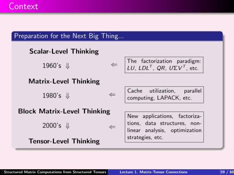
Context
Preparation for the Next Big Thing...
Scalar-Level Thinking
1960’s ⇓
Matrix-Level Thinking
1980’s ⇓
Block Matrix-Level Thinking
2000’s ⇓
Tensor-Level Thinking
⇐ The factorization paradigm:LU, LDLT , QR, UΣV T , etc.
⇐ Cache utilization, parallelcomputing, LAPACK, etc.
⇐New applications, factoriza-tions, data structures, non-linear analysis, optimizationstrategies, etc.
Structured Matrix Computations from Structured Tensors Lecture 1. Matrix-Tensor Connections 59 / 60
Page 60
More Context
A Changing Definition of “Big”
In Matrix Computations, to say that A ∈ IRn1×n2 is “big” is to saythat both n1 and n2 are big.
In Tensor Computations, to say that A ∈ IRn1×···×nd is “big” is to saythat n1n2 · · · nd is big and this need not require big nk . E.g.n1 = n2 = · · · = n1000 = 2.
Algorithms that scale with d will induce a transition...
Matrix-Based Scientific Computation
⇓Tensor-Based Scientific Computation
Structured Matrix Computations from Structured Tensors Lecture 1. Matrix-Tensor Connections 60 / 60