44
Modelling Modelling- Module 1 Module 1 Lecture 1 Lecture 1 David Godfrey
| Date post: | 09-Apr-2018 |
| Category: |
Documents |
| Upload: | chadwheeler |
| View: | 221 times |
| Download: | 0 times |
8/7/2019 Lecture 1 Module 1
http://slidepdf.com/reader/full/lecture-1-module-1 1/44
ModellingModelling-- Module 1Module 1
Lecture 1Lecture 1
David Godfrey
8/7/2019 Lecture 1 Module 1
http://slidepdf.com/reader/full/lecture-1-module-1 2/44
Slide number 2
Lecture 1 Introduction to ProcessLecture 1 Introduction to Process
Mathematical models
Building a model
Checking dimensional consistency Traffic light problem
8/7/2019 Lecture 1 Module 1
http://slidepdf.com/reader/full/lecture-1-module-1 3/44
Slide number 3
What is a Model?What is a Model?
Dictionary definition
³Imitation of something on asmaller scale´
8/7/2019 Lecture 1 Module 1
http://slidepdf.com/reader/full/lecture-1-module-1 4/44
Slide number 4
What is a Mathematical ModelWhat is a Mathematical Model
of a System?of a System?
A mathematical model is a set of
mathematical statements which
attempts to describe the system Usually the statements are
equations
8/7/2019 Lecture 1 Module 1
http://slidepdf.com/reader/full/lecture-1-module-1 5/44
Slide number 5
What is a System?...examplesWhat is a System?...examples
Flight of a ball
A yacht
A building The human body
An electric supply grid
8/7/2019 Lecture 1 Module 1
http://slidepdf.com/reader/full/lecture-1-module-1 6/44
Slide number 6
Why use Mathematical Models?Why use Mathematical Models?
A deeper understanding of thesystem is obtained and the laws of nature are often relevant, e.g.
Newton¶s laws of motion Enables systems to be designed
and/or modified without trial and
error on expensive full scalemodels, i.e. we can use computer models
8/7/2019 Lecture 1 Module 1
http://slidepdf.com/reader/full/lecture-1-module-1 7/44
Slide number 7
The Kiss PrincipleThe Kiss Principle
³Keep it simple stupid´
In practice models are very
simplified and often only attemptto model part of the system
Always start by considering the
simplest model, then add in
more complexities to make the
model more realistic
8/7/2019 Lecture 1 Module 1
http://slidepdf.com/reader/full/lecture-1-module-1 8/44
Slide number 8
How to Build a Mathematical ModelHow to Build a Mathematical Model
Identify the problem
Formulate a mathematicalmodel
Obtain a mathematical solution
Interpret the solution
Compare with reality
either Go back through the loop
or Write a report
8/7/2019 Lecture 1 Module 1
http://slidepdf.com/reader/full/lecture-1-module-1 9/44
Slide number 9
First Two StepsFirst Two Steps
Represent the physical factors bymathematical symbols (some will bevariables, including parameters, and
some will be constants) Make assumptions about how they
are related
Formulate a precise problemstatement
Formulate some equations
8/7/2019 Lecture 1 Module 1
http://slidepdf.com/reader/full/lecture-1-module-1 10/44
Slide number 10
Quantifiable FactorsQuantifiable Factors
Constants
Variables«input and output;
independent and dependant Parameters«fixed variables«often
fixed for this particular model and
often fixed to simplify the model
8/7/2019 Lecture 1 Module 1
http://slidepdf.com/reader/full/lecture-1-module-1 11/44
Slide number 11
Assumptions«about basic shapes Assumptions«about basic shapes
Perfect formation of shapes
Uniformity of thickness and density
Ignore extra material«at this stage
These assumptions ³allow´ us to use
standard formulae in our models
8/7/2019 Lecture 1 Module 1
http://slidepdf.com/reader/full/lecture-1-module-1 12/44
Slide number 12
Precise Problem StatementPrecise Problem Statement
Given (input, variables, parameters,constants) find (output, variables)such that (condition is satisfied or
objective is achieved. E.g. Given a fixed width piece of
metal find the dimensions such that
the maximum volume is obtainedwhen the metal is formed into a ³u´shaped gutter
8/7/2019 Lecture 1 Module 1
http://slidepdf.com/reader/full/lecture-1-module-1 13/44
Slide number 13
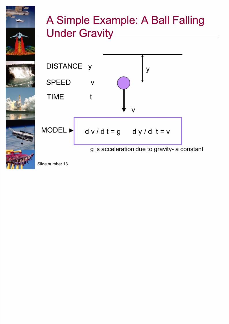
A Simple Example: A Ball Falling A Simple Example: A Ball Falling
Under GravityUnder Gravity
v
SPEED v
DISTANCE y y
TIME t
MODEL d v / d t = g
g is acceleration due to gravity- a constant
d y / d t = v
8/7/2019 Lecture 1 Module 1
http://slidepdf.com/reader/full/lecture-1-module-1 14/44
Slide number 14
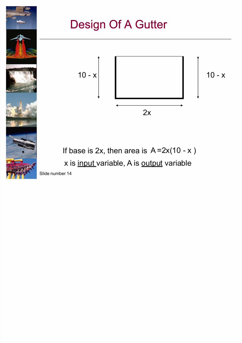
Design Of A Gutter Design Of A Gutter
10 - x 10 - x
2x
If base is 2x, then area is A =2x(10 - x )
x is input variable, A is output variable
8/7/2019 Lecture 1 Module 1
http://slidepdf.com/reader/full/lecture-1-module-1 15/44
Slide number 15
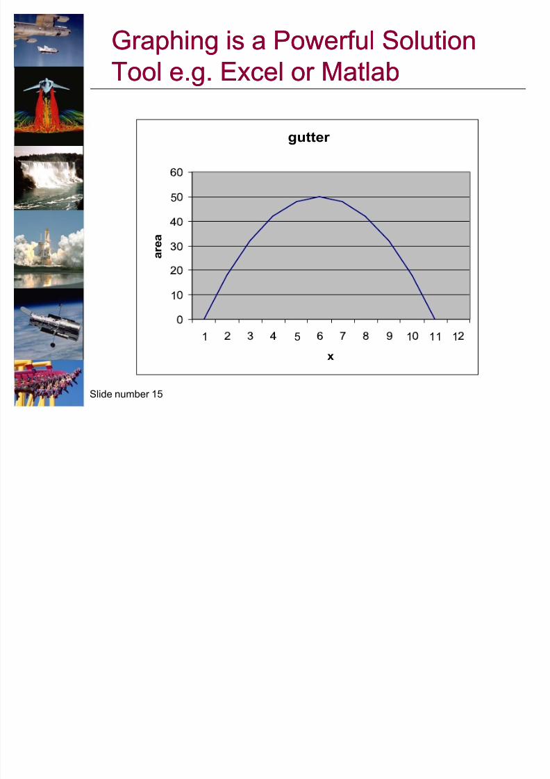
Graphing is a Powerful SolutionGraphing is a Powerful Solution
Tool e.g. Excel or MatlabTool e.g. Excel or Matlab
gutter
1
5
1 5 1 11 1
x
a r e a
8/7/2019 Lecture 1 Module 1
http://slidepdf.com/reader/full/lecture-1-module-1 16/44
Slide number 16
Some ChecksSome Checks
Are equations consistent ± it is
particularly important to check
that they are DIMENSIONALLY
CORRECT
It is also important to check the
qualitative behaviour
8/7/2019 Lecture 1 Module 1
http://slidepdf.com/reader/full/lecture-1-module-1 17/44
Slide number 17
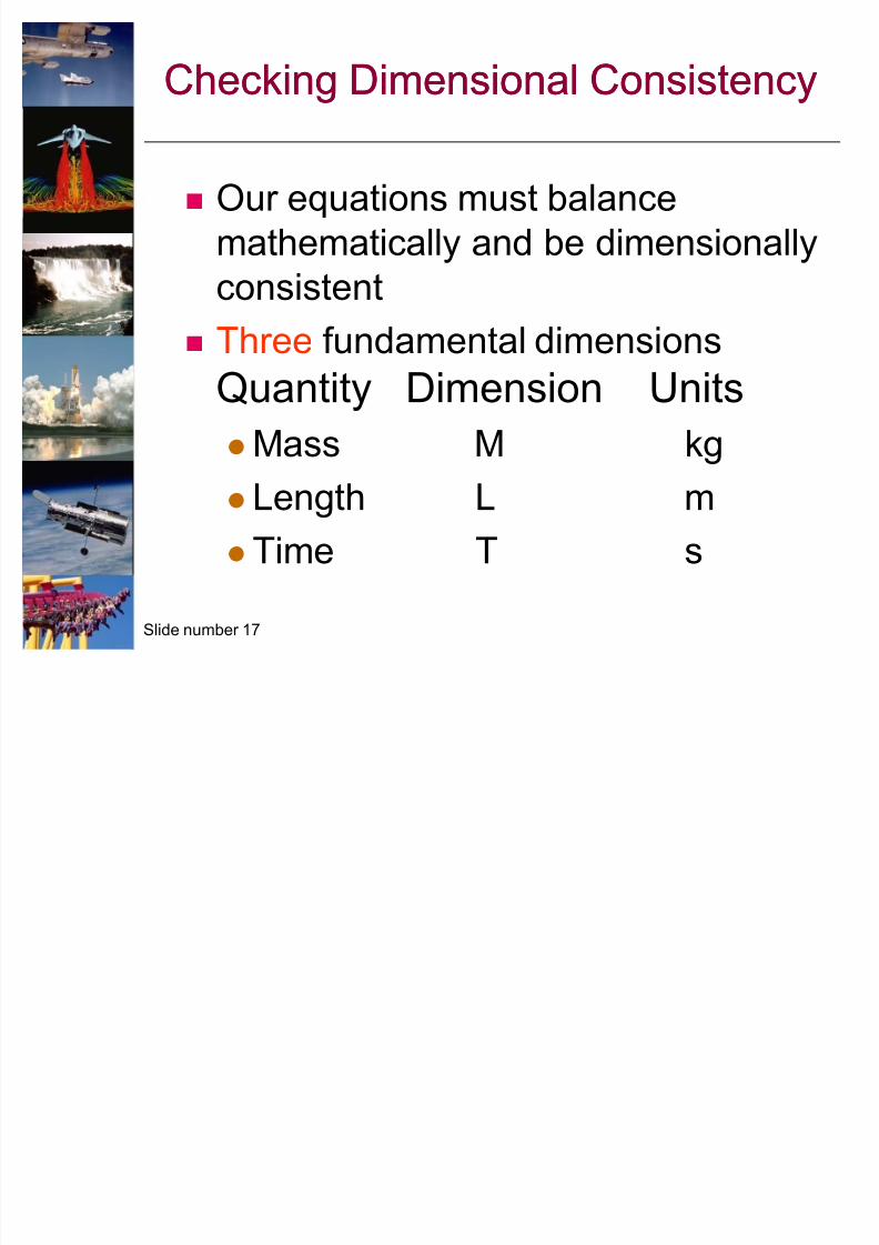
Checking Dimensional ConsistencyChecking Dimensional Consistency
Our equations must balance
mathematically and be dimensionally
consistent
Three fundamental dimensions
Quantity Dimension Units
Mass M kg Length L m
Time T s
8/7/2019 Lecture 1 Module 1
http://slidepdf.com/reader/full/lecture-1-module-1 18/44
Slide number 18
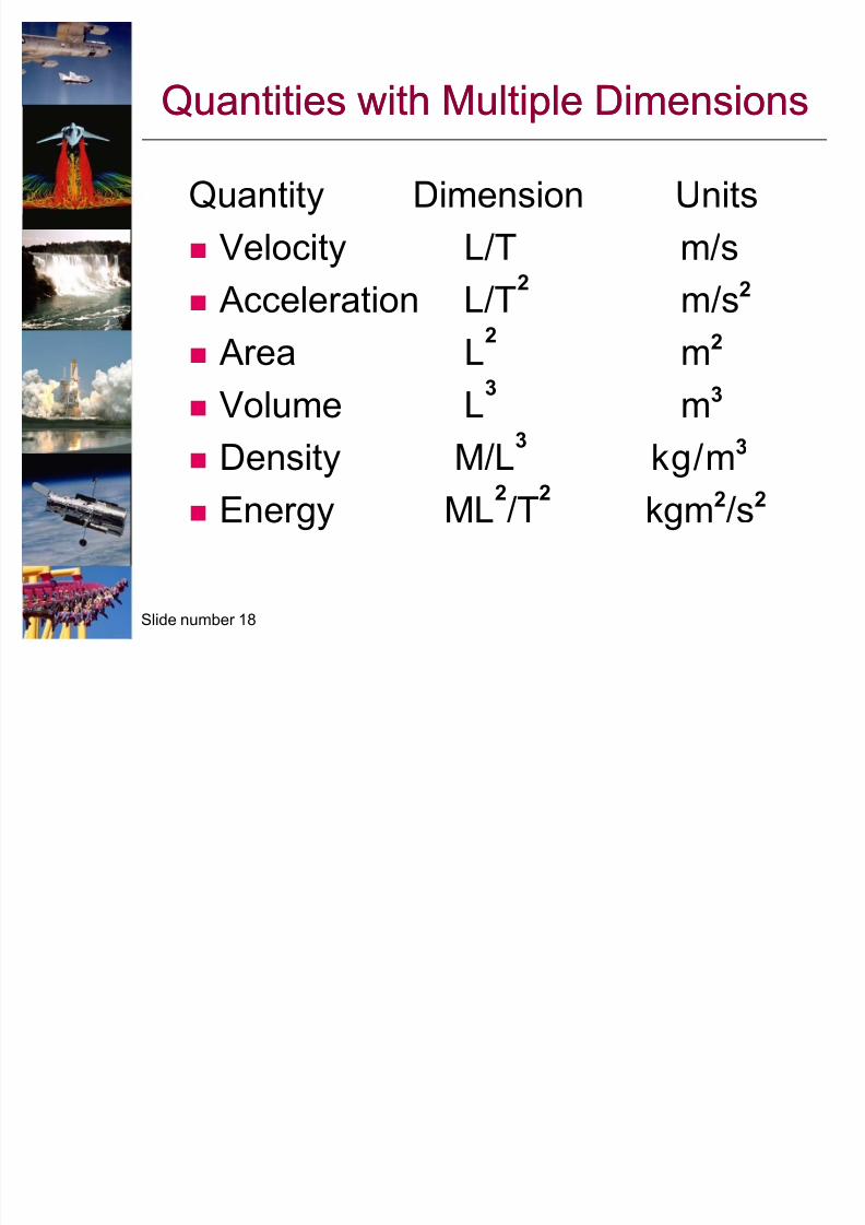
Quantities with Multiple DimensionsQuantities with Multiple Dimensions
Quantity Dimension Units
Velocity L/T m/s
Acceleration L/T2
m/s2
Area L2
m2
Volume L3
m3
Density M/L3
kg/m3
Energy ML2/T
2kgm2/s2
8/7/2019 Lecture 1 Module 1
http://slidepdf.com/reader/full/lecture-1-module-1 19/44
Slide number 19
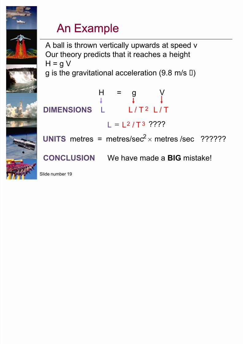
An Example An Example
A ball is thrown vertically upwards at speed vOur theory predicts that it reaches a height
H = g V
g is the gravitational acceleration (9.8 m/s )
H = g V
DIMENSIONS L
CONCLUSION We have made a BIG mistake!
L / T2L / T
????32
T/LL !UNITS metres = metres/sec v metres /sec ??????2
8/7/2019 Lecture 1 Module 1
http://slidepdf.com/reader/full/lecture-1-module-1 20/44
8/7/2019 Lecture 1 Module 1
http://slidepdf.com/reader/full/lecture-1-module-1 21/44
Slide number 21
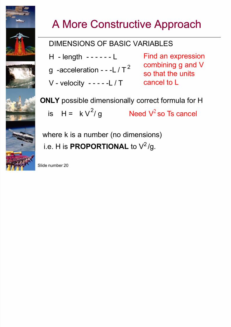
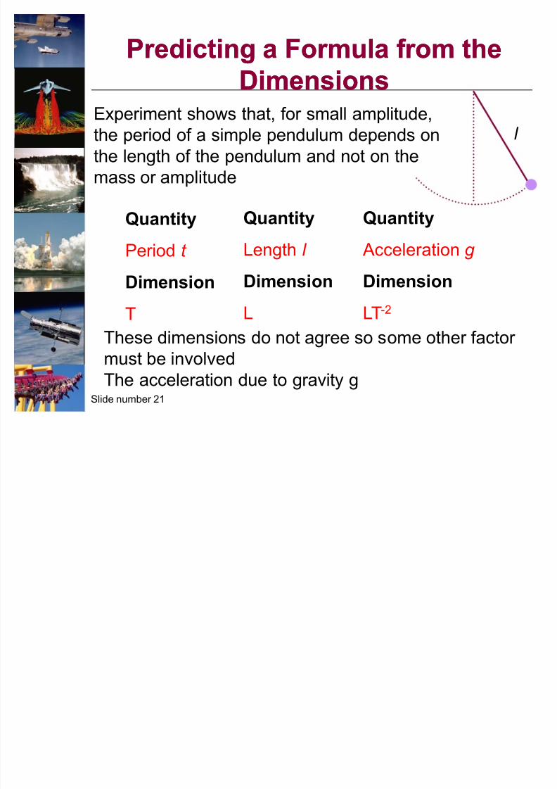
Predicting a Formula f r om the Predicting a Formula f r om the
DimensionsDimensionsExperiment shows that, for small amplitude,
the period of a simple pendulum depends on
the length of the pendulum and not on the
mass or amplitude
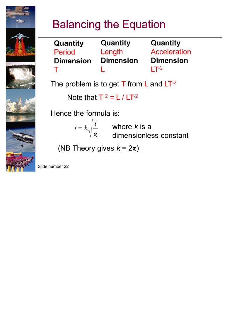
Quantity
Period t
Dimension
T
Quantity
Length l
Dimension
L
These dimensions do not agree so some other factor
must be involved
The acceleration due to gravity g
Quantity
Acceleration g
Dimension
LT-2
l
8/7/2019 Lecture 1 Module 1
http://slidepdf.com/reader/full/lecture-1-module-1 22/44
8/7/2019 Lecture 1 Module 1
http://slidepdf.com/reader/full/lecture-1-module-1 23/44
Slide number 23
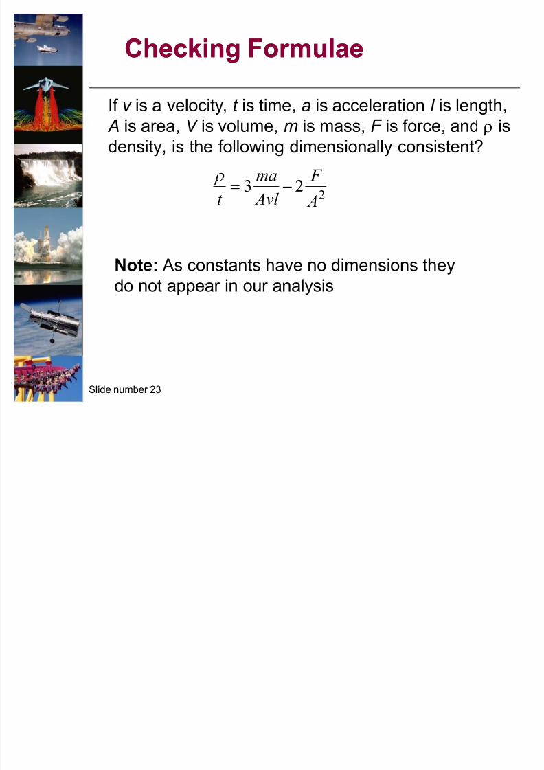
Checking FormulaeChecking Formulae
If v is a velocity, t is time, a is acceleration l is length,
A is area, V is volume, m is mass, F is force, and V is
density, is the following dimensionally consistent?
Note: As constants have no dimensions they
do not appear in our analysis
223
A
F
Avl
ma
t !
V
8/7/2019 Lecture 1 Module 1
http://slidepdf.com/reader/full/lecture-1-module-1 24/44
Slide number 24
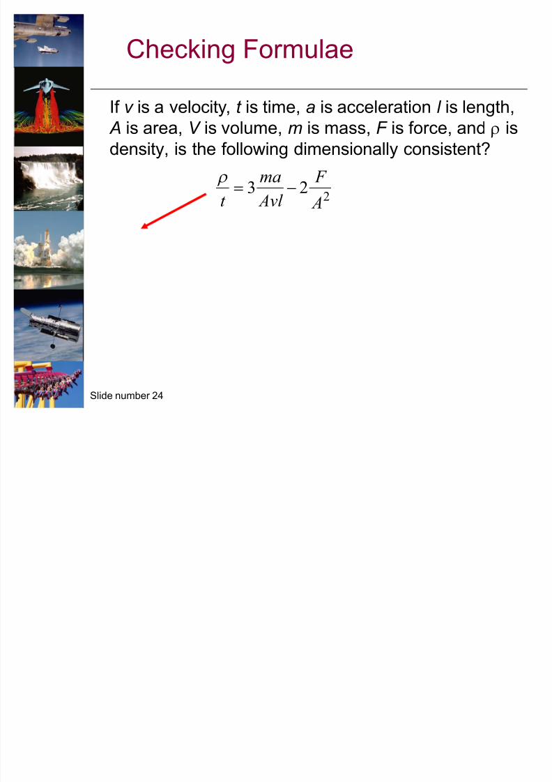
Checking Formulae
If v is a velocity, t is time, a is acceleration l is length,
A is area, V is volume, m is mass, F is force, and V is
density, is the following dimensionally consistent?
13
3
TML
T
1
L
M
!
223
A
F
Avl
ma
t !
V
8/7/2019 Lecture 1 Module 1
http://slidepdf.com/reader/full/lecture-1-module-1 25/44
Slide number 25
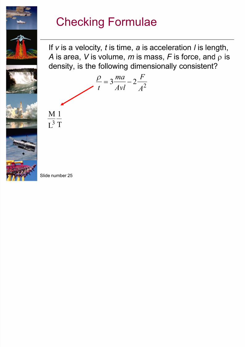
Checking Formulae
If v is a velocity, t is time, a is acceleration l is length,
A is area, V is volume, m is mass, F is force, and V is
density, is the following dimensionally consistent?
13
3
T
T
1
L
M
!
2
23
A
F
Avl
ma
t !
V

8/7/2019 Lecture 1 Module 1
http://slidepdf.com/reader/full/lecture-1-module-1 26/44
Slide number 26
Checking Formulae
If v is a velocity, t is time, a is acceleration l is length,
A is area, V is volume, m is mass, F is force, and V is
density, is the following dimensionally consistent?
13
3
TML
T
1
L
M
!
2
23
A
F
Avl
ma
t !
V
8/7/2019 Lecture 1 Module 1
http://slidepdf.com/reader/full/lecture-1-module-1 27/44
Slide number 27
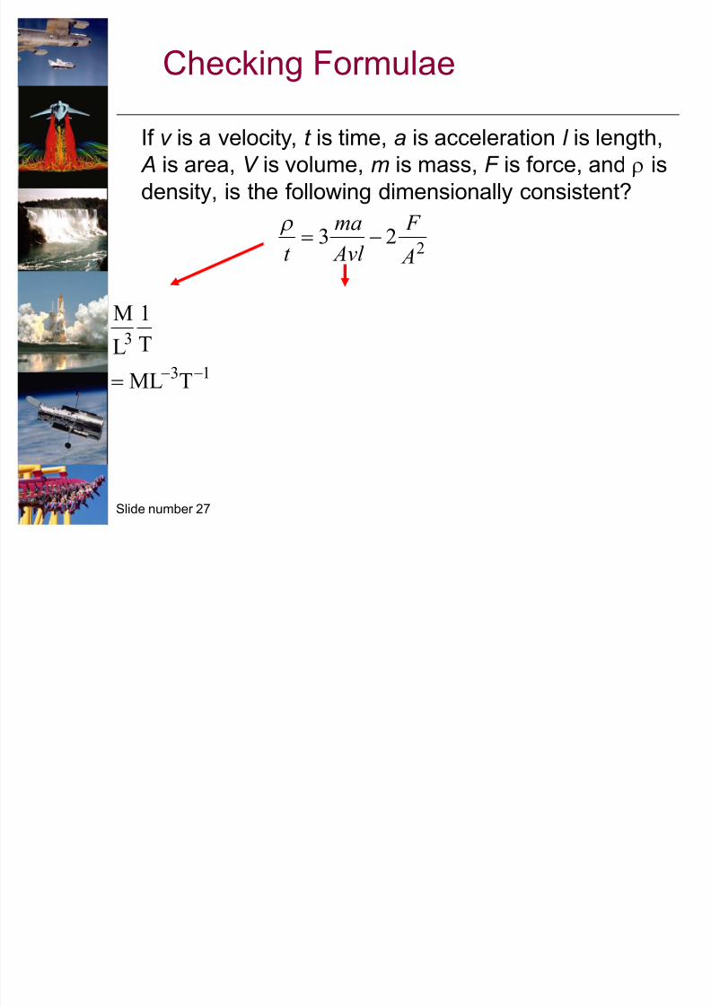
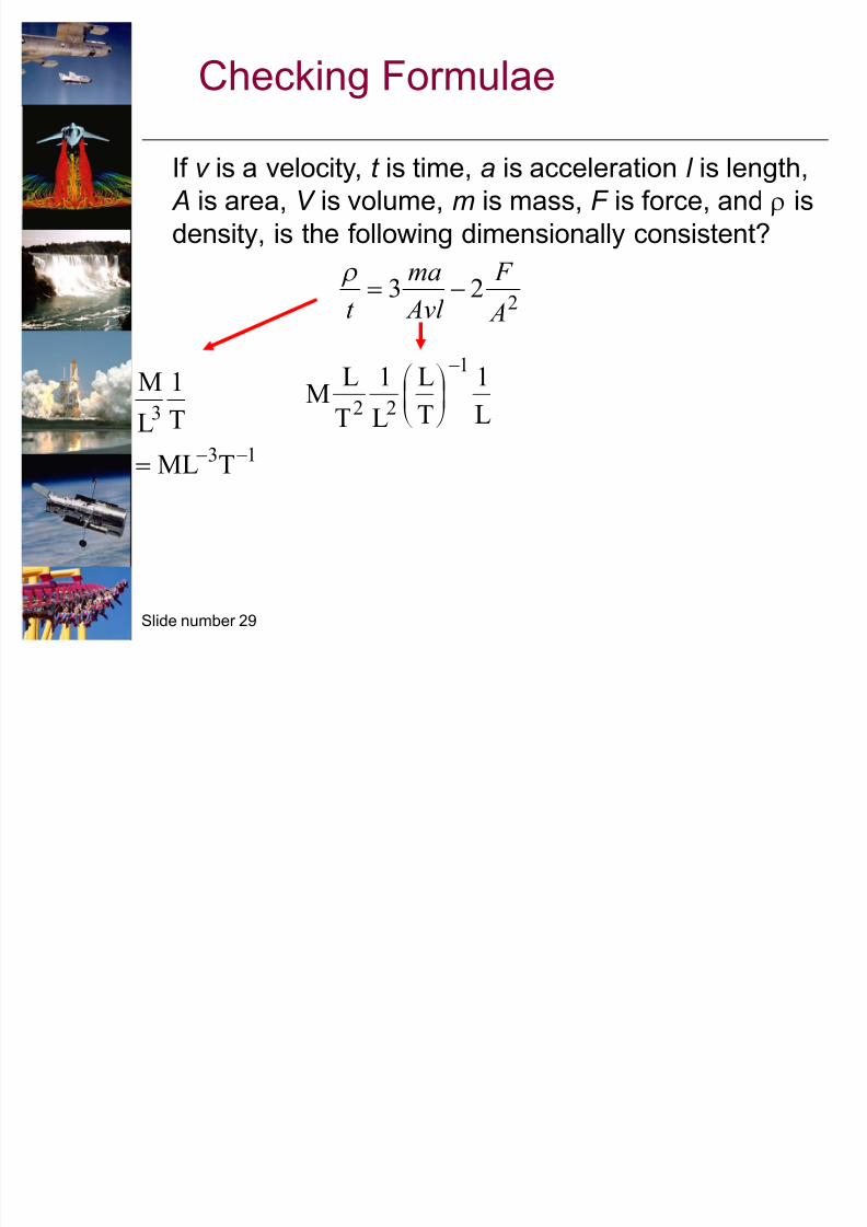
Checking Formulae
If v is a velocity, t is time, a is acceleration l is length,
A is area, V is volume, m is mass, F is force, and V is
density, is the following dimensionally consistent?
13
3
TML
T
1
L
M
!13
1122
1
22
TML
TLLMT
T
L
L
1
T
LM
!!
¹ º ¸
©ª¨
2
23
A
F
Avl
ma
t !
V
8/7/2019 Lecture 1 Module 1
http://slidepdf.com/reader/full/lecture-1-module-1 28/44
Slide number 28
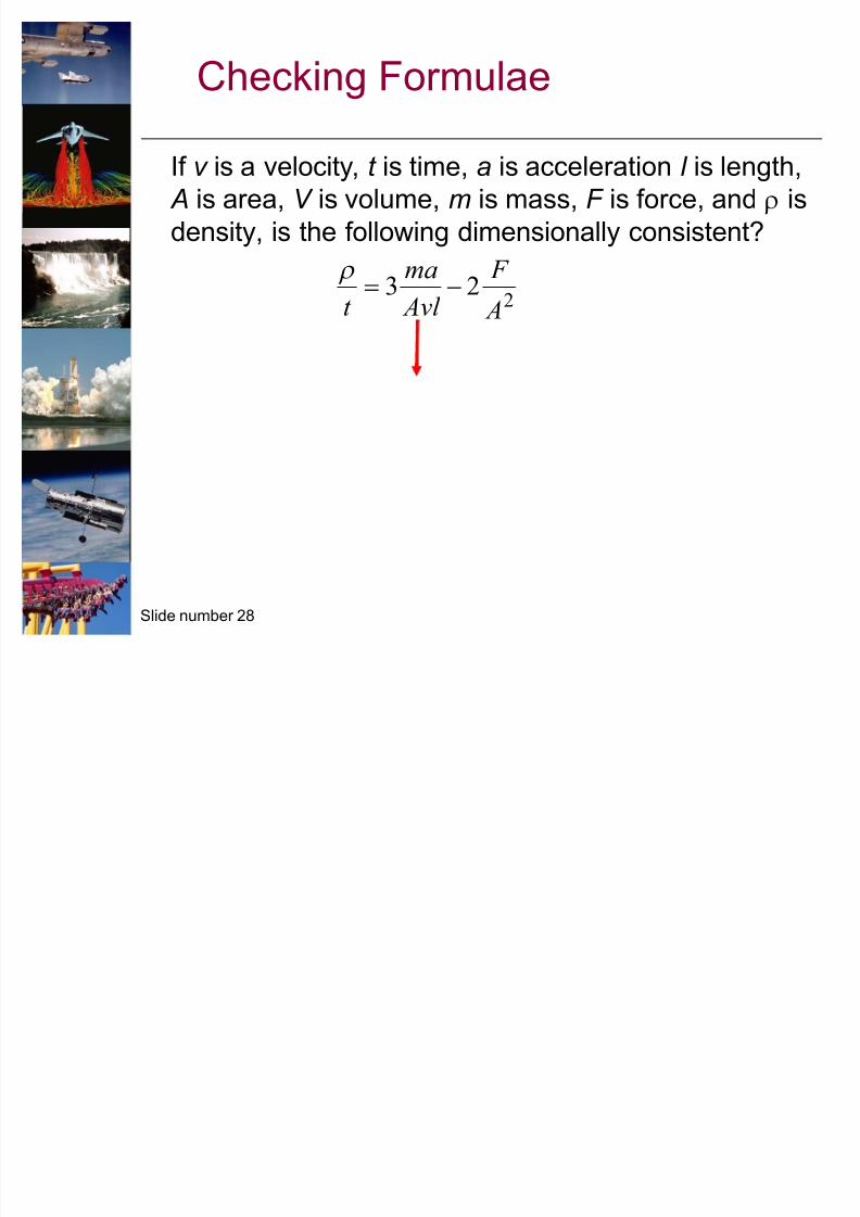
Checking Formulae
If v is a velocity, t is time, a is acceleration l is length,
A is area, V is volume, m is mass, F is force, and V is
density, is the following dimensionally consistent?
2
23
A
F
Avl
ma
t !
V
8/7/2019 Lecture 1 Module 1
http://slidepdf.com/reader/full/lecture-1-module-1 29/44

8/7/2019 Lecture 1 Module 1
http://slidepdf.com/reader/full/lecture-1-module-1 30/44
Slide number 30
13
1-1122
1
22
TML
LTLLMLT
L
1
T
L
L
1
T
LM
!
!
¹ º ¸
©ª¨
Checking Formulae
If v is a velocity, t is time, a is acceleration i is length,
A is area, V is volume, m is mass, F is force, and V is
density, is the following dimensionally consistent?
13
3
TML
T
1
L
M
!
2
23
A
F
Avl
ma
t !
V

8/7/2019 Lecture 1 Module 1
http://slidepdf.com/reader/full/lecture-1-module-1 31/44
Slide number 31
Checking Formulae
If v is a velocity, t is time, a is acceleration i is length,
A is area, V is volume, m is mass, F is force, and V is
density, is the following dimensionally consistent?
13
3
TML
T
1
L
M
!
2
23
A
F
Avl
ma
t !
V
13
1-1122
1
22
TML
LTLLMLT
L
1
T
L
L
1
T
LM
!
!
¹ º ¸
©ª¨
8/7/2019 Lecture 1 Module 1
http://slidepdf.com/reader/full/lecture-1-module-1 32/44
Slide number 32
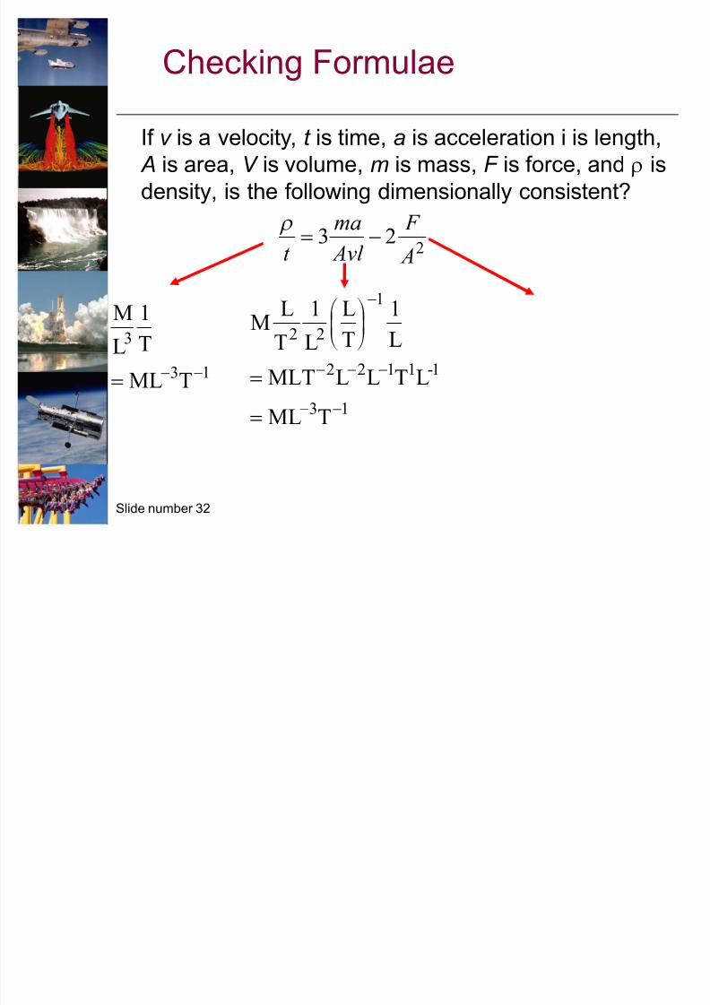
Checking Formulae
If v is a velocity, t is time, a is acceleration i is length,
A is area, V is volume, m is mass, F is force, and V is
density, is the following dimensionally consistent?
13
3
TML
T
1
L
M
!
32
42
22
2
LMT
LMLT
L
1
T
LM
!
!
2
23
A
F
Avl
ma
t !
V
13
1-1122
1
22
TML
LTLLMLT
L
1
T
L
L
1
T
LM
!
!
¹ º ¸
©ª¨
8/7/2019 Lecture 1 Module 1
http://slidepdf.com/reader/full/lecture-1-module-1 33/44
Slide number 33
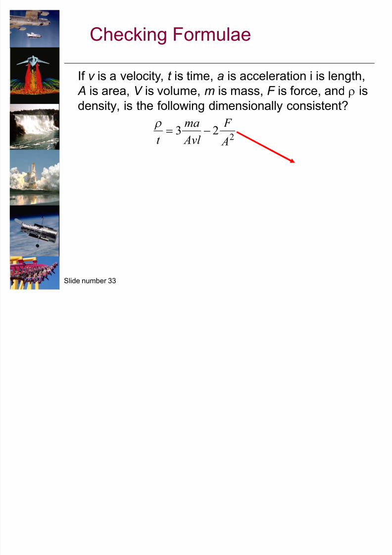
Checking Formulae
If v is a velocity, t is time, a is acceleration i is length,
A is area, V is volume, m is mass, F is force, and V is
density, is the following dimensionally consistent?
32
42
22
2
LMT
LMLT
L
1
T
LM
!
!
2
23
A
F
Avl
ma
t !
V
8/7/2019 Lecture 1 Module 1
http://slidepdf.com/reader/full/lecture-1-module-1 34/44
Slide number 34
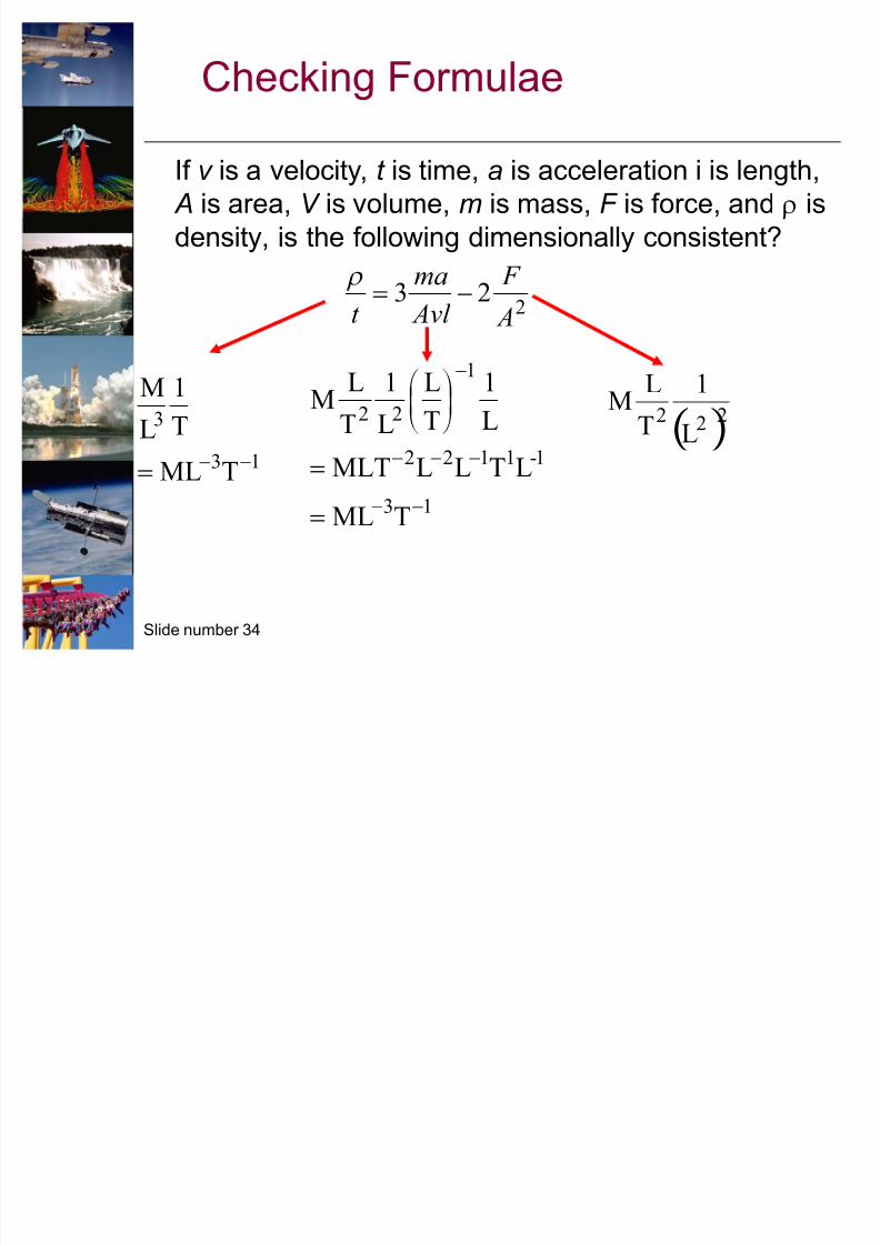
Checking Formulae
If v is a velocity, t is time, a is acceleration i is length,
A is area, V is volume, m is mass, F is force, and V is
density, is the following dimensionally consistent?
13
3
TML
T
1
L
M
!
32
42
22
2
LMT
LMLT
L
1
T
LM
!
!
2
23
A
F
Avl
ma
t !
V
13
1-1122
1
22
TML
LTLLMLT
L
1
T
L
L
1
T
LM
!
!
¹ º ¸
©ª¨
8/7/2019 Lecture 1 Module 1
http://slidepdf.com/reader/full/lecture-1-module-1 35/44
Slide number 35
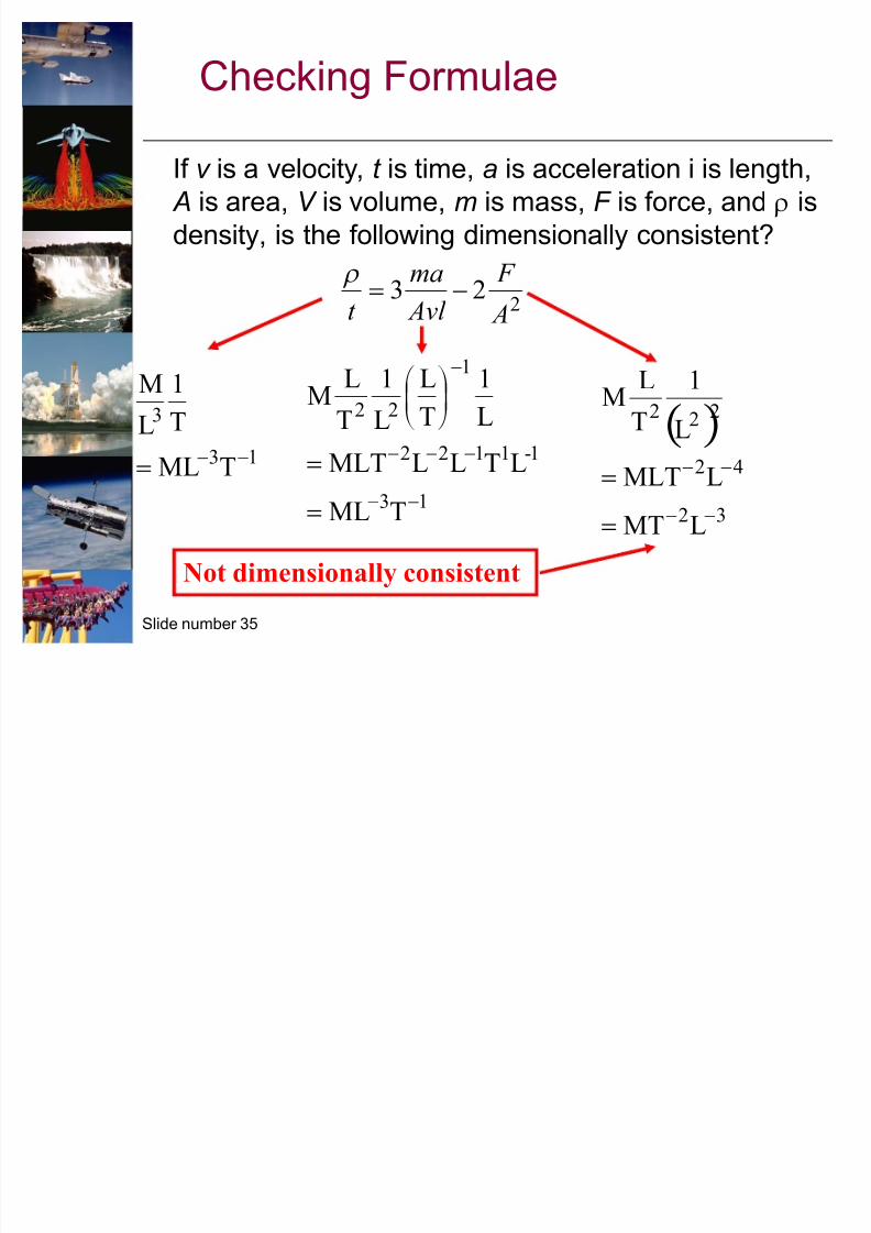
Checking Formulae
If v is a velocity, t is time, a is acceleration i is length,
A is area, V is volume, m is mass, F is force, and V is
density, is the following dimensionally consistent?
13
3
TML
T
1
L
M
!
32
42
22
2
LMT
LMLT
L
1
T
LM
!
!
Not dimensionally consistent
2
23
A
F
Avl
ma
t !
V
13
1-1122
1
22
TML
LTLLMLT
L
1
T
L
L
1
T
LM
!
!
¹ º ¸
©ª¨
8/7/2019 Lecture 1 Module 1
http://slidepdf.com/reader/full/lecture-1-module-1 36/44
Slide number 36
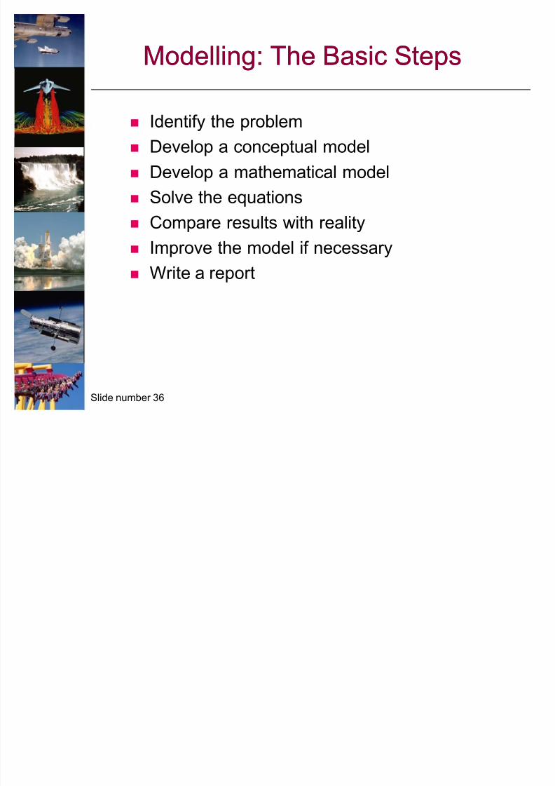
Modelling: The Basic StepsModelling: The Basic Steps
Identify the problem
Develop a conceptual model
Develop a mathematical model
Solve the equations Compare results with reality
Improve the model if necessary
Write a report
8/7/2019 Lecture 1 Module 1
http://slidepdf.com/reader/full/lecture-1-module-1 37/44
Slide number 37
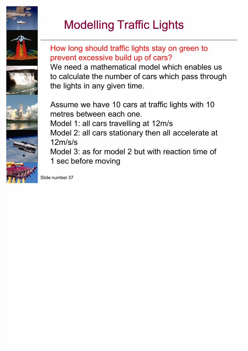
Modelling Traffic LightsModelling Traffic Lights
How long should traffic lights stay on green to
prevent excessive build up of cars?
We need a mathematical model which enables us
to calculate the number of cars which pass through
the lights in any given time.
Assume we have 10 cars at traffic lights with 10
metres between each one.
Model 1: all cars travelling at 12m/s
Model 2: all cars stationary then all accelerate at12m/s/s
Model 3: as for model 2 but with reaction time of
1 sec before moving
8/7/2019 Lecture 1 Module 1
http://slidepdf.com/reader/full/lecture-1-module-1 38/44
Slide number 38
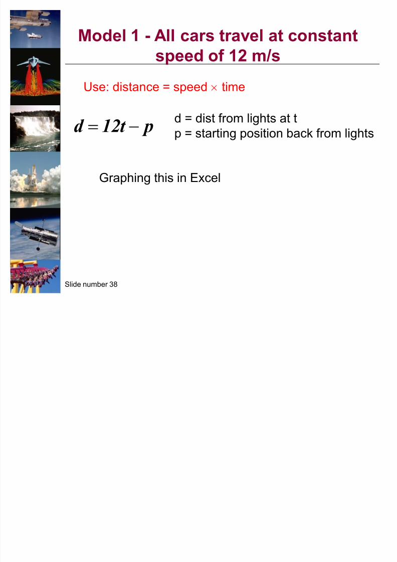
Model 1 - All cars tr avel at constant
speed of 12 m/s
d = dist from lights at t
p = starting position back from lights
Use: distance = speed v time
Graphing this in Excel
pt 12d !
8/7/2019 Lecture 1 Module 1
http://slidepdf.com/reader/full/lecture-1-module-1 39/44
Slide number 39
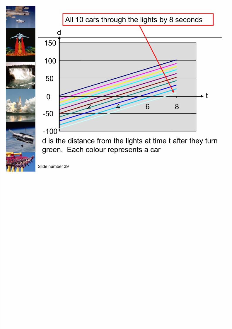
-100
-50
0
50
100
150
2 4 6 8
t
d
d is the distance from the lights at time t after they turn
green. Each colour represents a car
All 10 cars through the lights by 8 seconds
8/7/2019 Lecture 1 Module 1
http://slidepdf.com/reader/full/lecture-1-module-1 40/44
Slide number 40
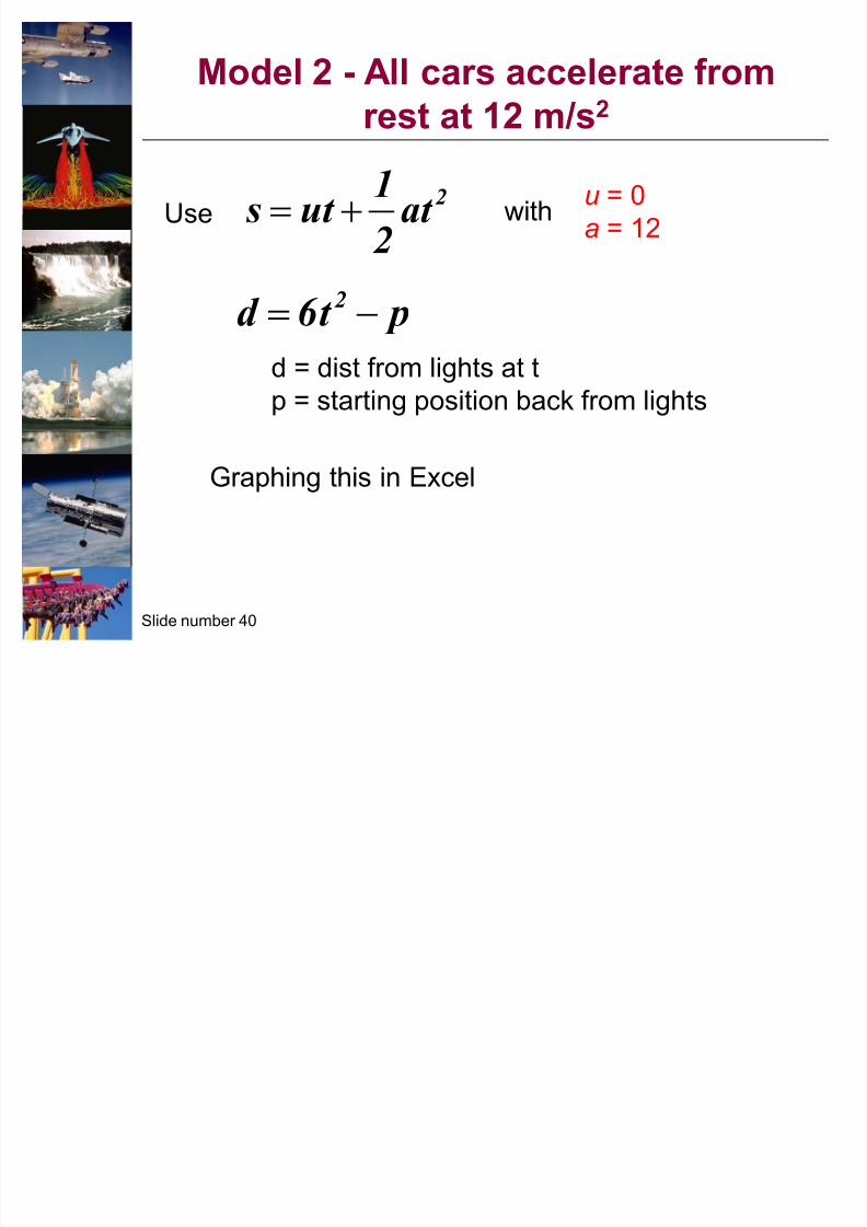
Model 2 - All cars acceler ate f r om
rest at 12 m/s2
u = 0
a = 12
Graphing this in Excel
2at
2
1ut s !Use
pt 6 d 2 !
d = dist from lights at t
p = starting position back from lights
with
8/7/2019 Lecture 1 Module 1
http://slidepdf.com/reader/full/lecture-1-module-1 41/44
Slide number 41
-100
-50
0
50
100
150
1 2 3 4
t
d
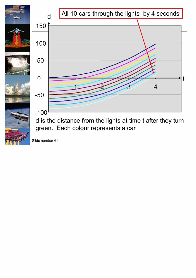
d is the distance from the lights at time t after they turn
green. Each colour represents a car
All 10 cars through the lights by 4 seconds
8/7/2019 Lecture 1 Module 1
http://slidepdf.com/reader/full/lecture-1-module-1 42/44
Slide number 42
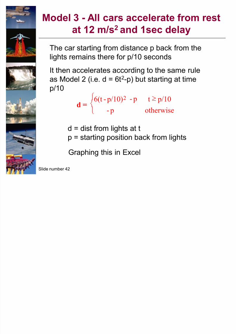
Model 3 - All cars acceler ate f r om rest
at 12 m/s2 and 1sec delay
d =
d = dist from lights at t
p = starting position back from lights
The car starting from distance p back from the
lights remains there for p/10 seconds
It then accelerates according to the same rule
as Model 2 (i.e. d = 6t2-p) but starting at time
p/10
°¯® u
otherwise p-
p/10t p/10)-6(t 2 p-
Graphing this in Excel
8/7/2019 Lecture 1 Module 1
http://slidepdf.com/reader/full/lecture-1-module-1 43/44
Slide number 43
-200
0
200
400
600
800
1000
2 4 6 8 10 12
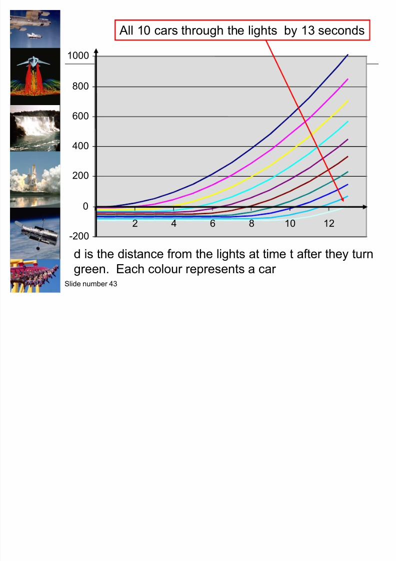
d is the distance from the lights at time t after they turn
green. Each colour represents a car
All 10 cars through the lights by 13 seconds
8/7/2019 Lecture 1 Module 1
http://slidepdf.com/reader/full/lecture-1-module-1 44/44
Slide number 44
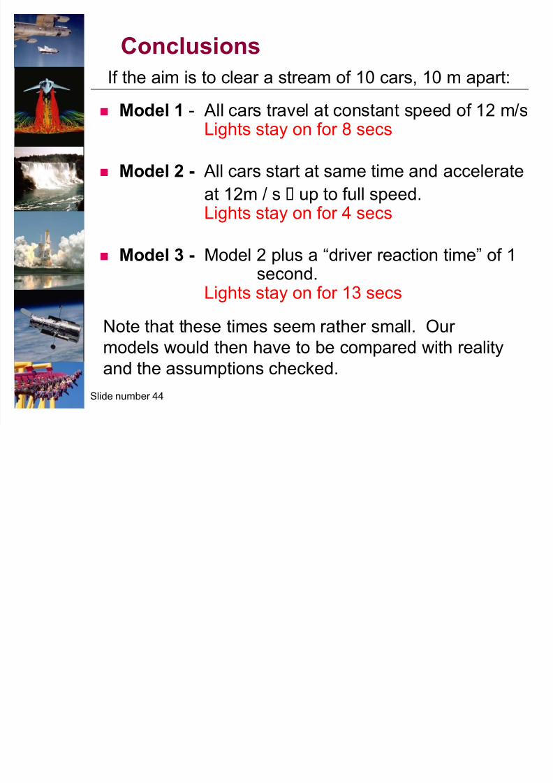
Model 1 - All cars travel at constant speed of 12 m/sLights stay on for 8 secs
Model 2 - All cars start at same time and accelerate
at 12m / s up to full speed.Lights stay on for 4 secs
Model 3 - Model 2 plus a ³driver reaction time´ of 1second.
Lights stay on for 13 secs
Conclusions
If the aim is to clear a stream of 10 cars, 10 m apart:
Note that these times seem rather small. Our
models would then have to be compared with reality
and the assumptions checked.


