67
Lecture 1: R Basics Jing Li http://cbb.sjtu.edu.cn/~jingli/ Dept of Bioinformatics & Biostatistics, SJTU [email protected]
| Date post: | 17-Dec-2015 |
| Category: |
Documents |
| Upload: | chastity-jemimah-kelley |
| View: | 225 times |
| Download: | 3 times |
Lecture 1: R Basics
Jing Lihttp://cbb.sjtu.edu.cn/~jingli/
Dept of Bioinformatics & Biostatistics, SJTU
2
Objectives
R basics R graph & data displaying Descriptive statistics and statistical inference
with R. Perform standard statistical analyses with R.
Textbooks
R for Beginners, Emmanuel Paradis
An Introduction to R, W. N. Venables, D. M. Smith and the R Development Core Team
Statistics with R, Vincent Zoonekynd
Grading
• Class participation 10%• Practice report 20%• Group presentation 20%• Final exam 40%

Contents (group work)
1. R basics 2. R graph3. Descriptive statistics and data displaying 4. T-test, ANOVA 5. Practice outside of class 6. Linear regression& correlation7. Chi-squared test8. Logistic regression & survival analysis 9. Non-parameter tests

Applied Statistical Computing and Graphics 6
Group presentation
30 min+ 15 Q&A (two or more member)
Role of each member
Submit ppt file by Thursday
7
Last class
R basic
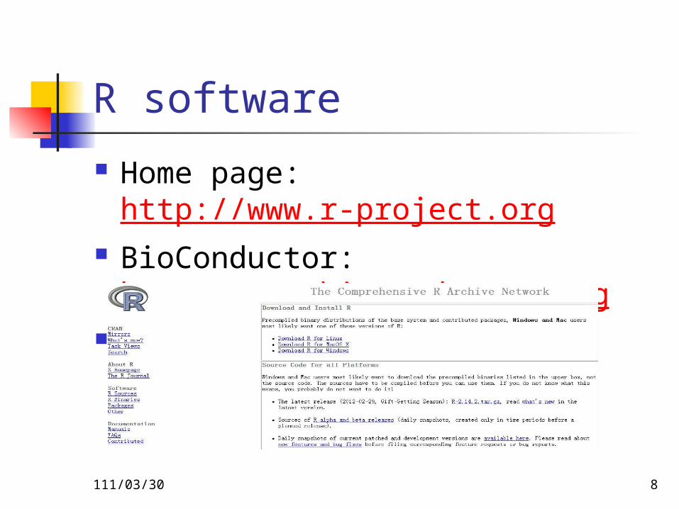
R software
Home page: http://www.r-project.org
BioConductor: http://www.bioconductor.org
For Linux/OS X/Windows
112/04/18 8
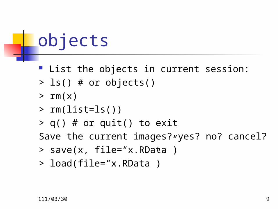
objects List the objects in current session:> ls() # or objects()> rm(x)> rm(list=ls())> q() # or quit() to exitSave the current images? yes? no? cancel?> save(x, file=“x.RData”)> load(file=“x.RData”)
112/04/18 9
112/04/18 10
Vectorized Arithmetic
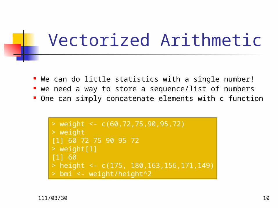
We can do little statistics with a single number! we need a way to store a sequence/list of numbers One can simply concatenate elements with c function
> weight <- c(60,72,75,90,95,72)> weight[1] 60 72 75 90 95 72> weight[1][1] 60> height <- c(175, 180,163,156,171,149)> bmi <- weight/height^2
112/04/18 11
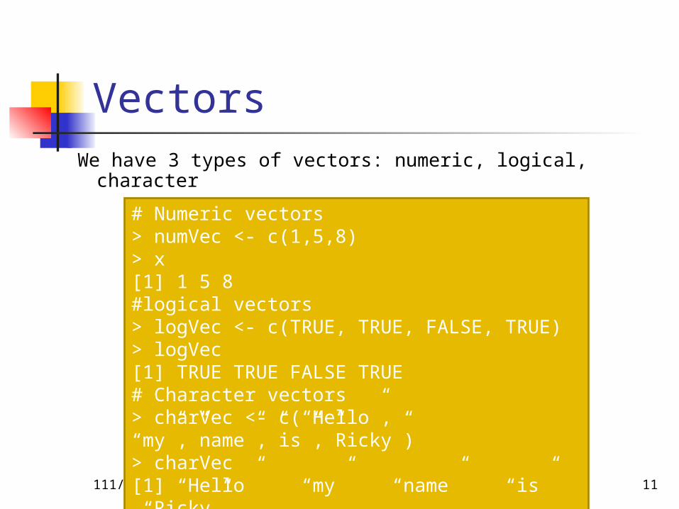
VectorsWe have 3 types of vectors: numeric, logical, character
# Numeric vectors> numVec <- c(1,5,8)> x[1] 1 5 8#logical vectors> logVec <- c(TRUE, TRUE, FALSE, TRUE)> logVec[1] TRUE TRUE FALSE TRUE# Character vectors> charVec <- c(“Hello”, “my”,”name”,”is”,”Ricky”)> charVec[1] “Hello” “my” “name” “is” “Ricky”
112/04/18 12
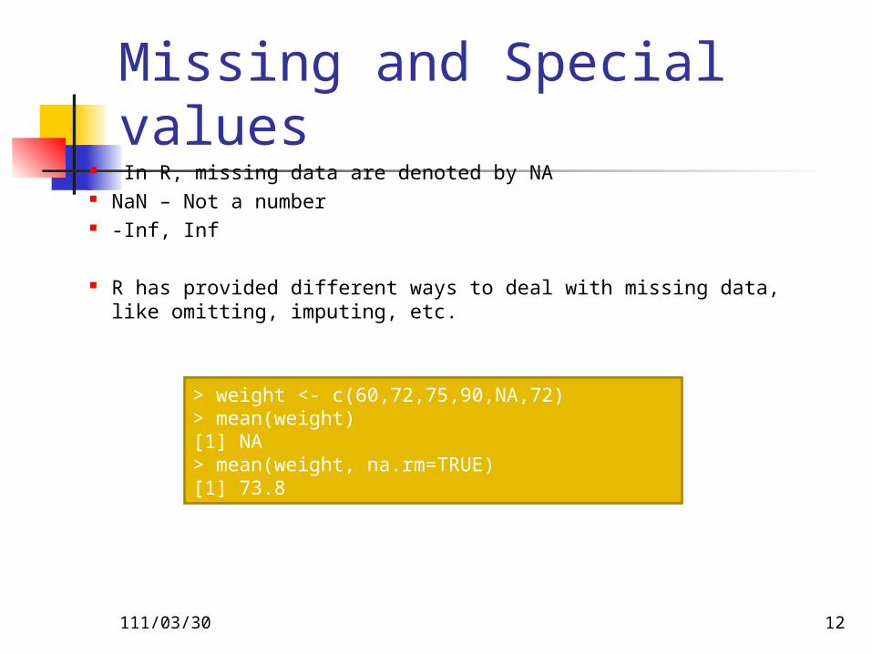
Missing and Special values In R, missing data are denoted by NA NaN – Not a number -Inf, Inf
R has provided different ways to deal with missing data, like omitting, imputing, etc.
> weight <- c(60,72,75,90,NA,72)> mean(weight)[1] NA> mean(weight, na.rm=TRUE)[1] 73.8
112/04/18 13
Matrices and arrays
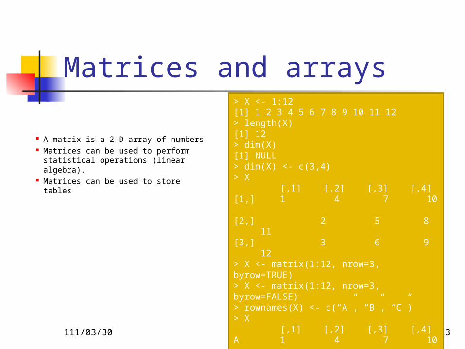
A matrix is a 2-D array of numbers Matrices can be used to perform
statistical operations (linear algebra).
Matrices can be used to store tables
> X <- 1:12[1] 1 2 3 4 5 6 7 8 9 10 11 12> length(X)[1] 12> dim(X)[1] NULL> dim(X) <- c(3,4)> X
[,1] [,2] [,3] [,4][1,] 1 4 7 10 [2,] 2 5 8 11[3,] 3 6 9 12> X <- matrix(1:12, nrow=3, byrow=TRUE)> X <- matrix(1:12, nrow=3, byrow=FALSE)> rownames(X) <- c(“A”, “B”, “C”)> X
[,1] [,2] [,3] [,4]A 1 4 7 10 B 2 5 8 11C 3 6 9 12> colnames(X) <- c(‘1’,’2’,’x’,’y’)> X
112/04/18 14
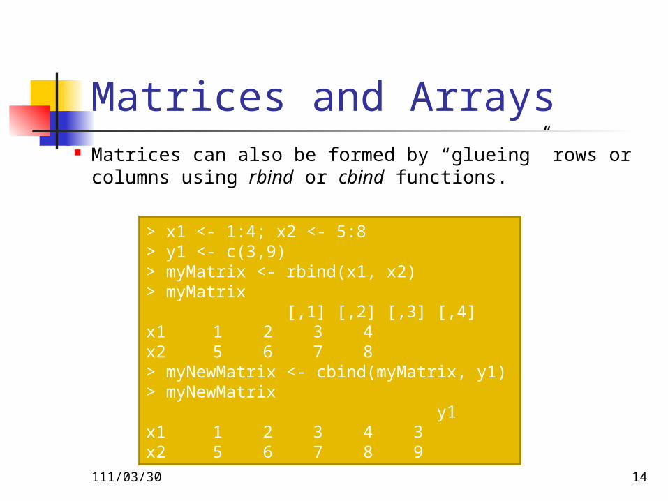
Matrices and Arrays Matrices can also be formed by “glueing” rows
or columns using rbind or cbind functions.
> x1 <- 1:4; x2 <- 5:8> y1 <- c(3,9)> myMatrix <- rbind(x1, x2)> myMatrix [,1] [,2] [,3] [,4]x1 1 2 3 4x2 5 6 7 8> myNewMatrix <- cbind(myMatrix, y1)> myNewMatrix y1x1 1 2 3 4 3x2 5 6 7 8 9
112/04/18 15
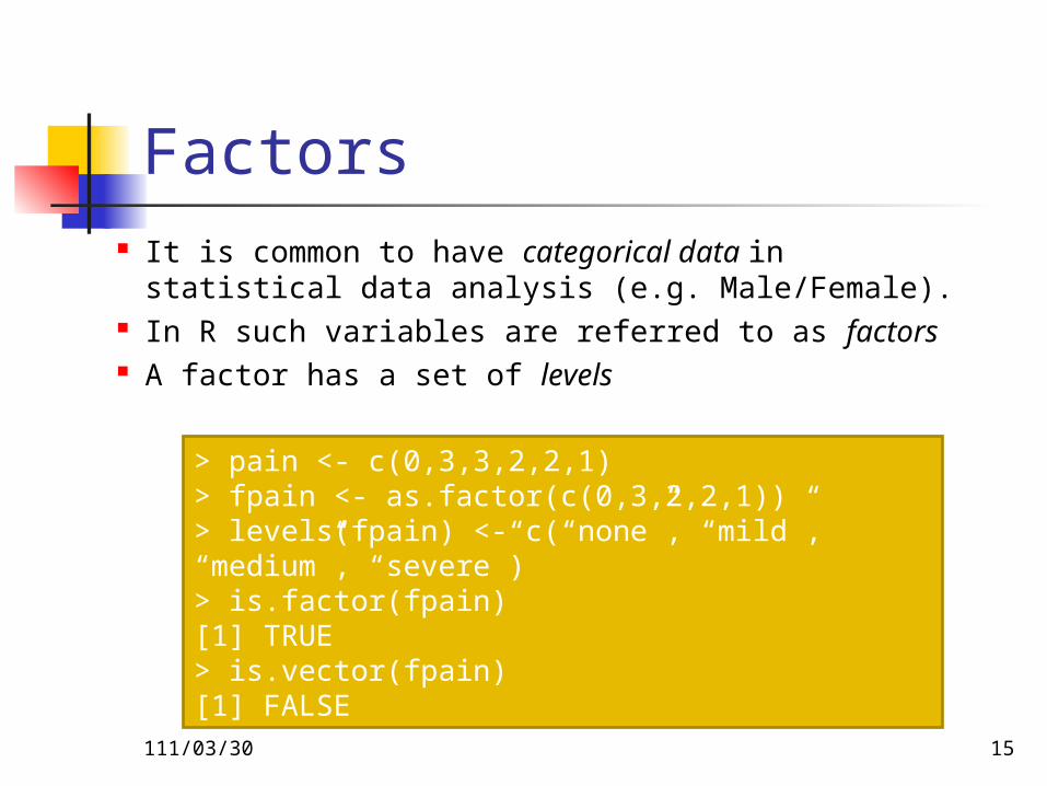
Factors It is common to have categorical data in
statistical data analysis (e.g. Male/Female). In R such variables are referred to as factors A factor has a set of levels
> pain <- c(0,3,3,2,2,1)> fpain <- as.factor(c(0,3,2,2,1))> levels(fpain) <- c(“none”, “mild”, “medium”, “severe”)> is.factor(fpain)[1] TRUE> is.vector(fpain)[1] FALSE
112/04/18 16
Lists
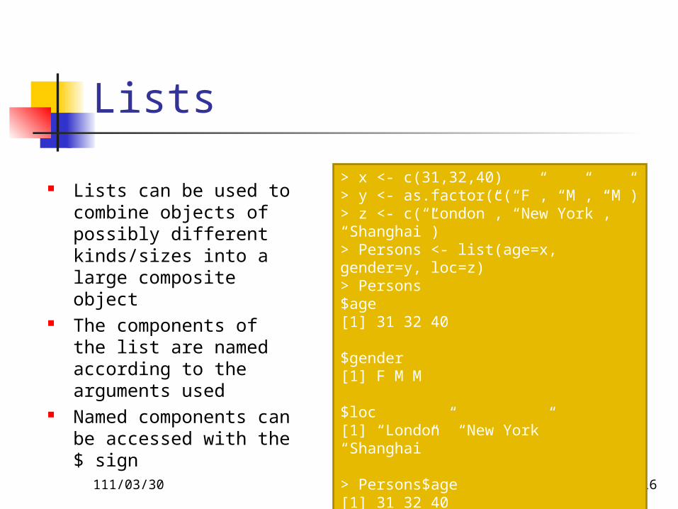
Lists can be used to combine objects of possibly different kinds/sizes into a large composite object
The components of the list are named according to the arguments used
Named components can be accessed with the $ sign
> x <- c(31,32,40)> y <- as.factor(c(“F”, “M”, “M”)> z <- c(“London”, “New York”, “Shanghai”)> Persons <- list(age=x, gender=y, loc=z)> Persons$age[1] 31 32 40
$gender[1] F M M
$loc[1] “London” “New York” “Shanghai”
> Persons$age[1] 31 32 40
112/04/18 17
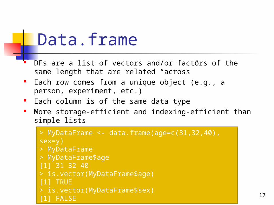
Data.frame DFs are a list of vectors and/or factors of the same length
that are related “across” Each row comes from a unique object (e.g., a person,
experiment, etc.) Each column is of the same data type More storage-efficient and indexing-efficient than simple
lists > MyDataFrame <- data.frame(age=c(31,32,40), sex=y)> MyDataFrame> MyDataFrame$age[1] 31 32 40> is.vector(MyDataFrame$age)[1] TRUE> is.vector(MyDataFrame$sex)[1] FALSE
112/04/18 18
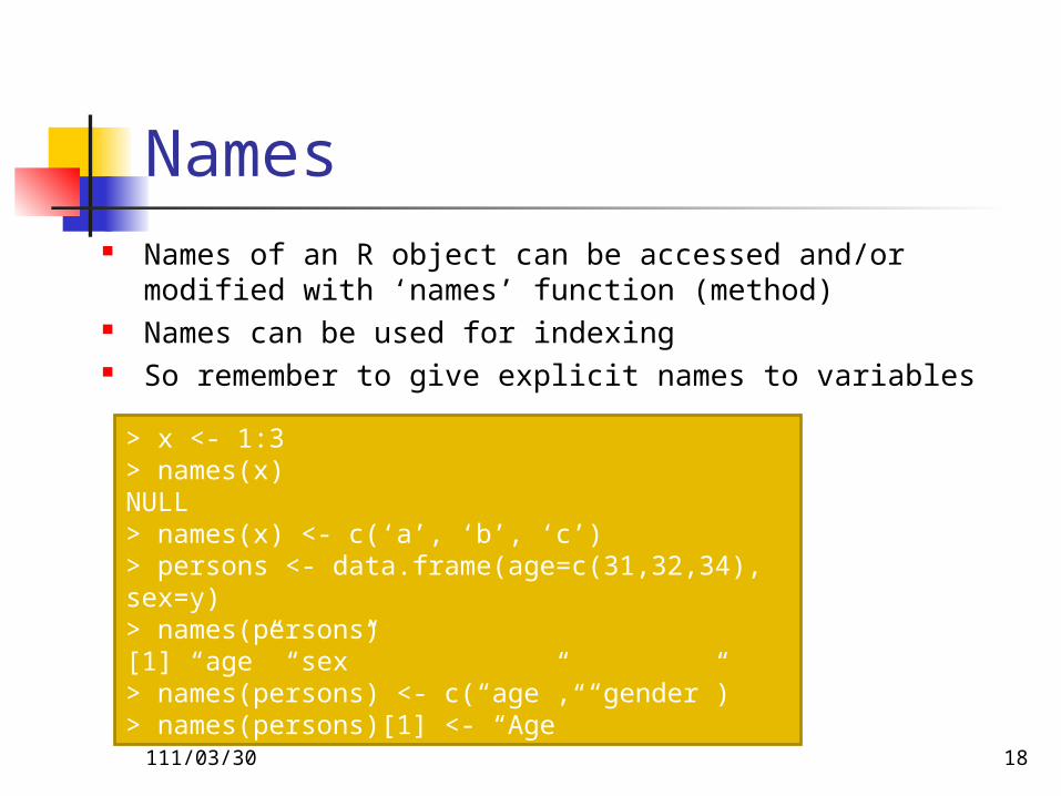
Names Names of an R object can be accessed and/or modified
with ‘names’ function (method) Names can be used for indexing So remember to give explicit names to variables
> x <- 1:3> names(x)NULL> names(x) <- c(‘a’, ‘b’, ‘c’)> persons <- data.frame(age=c(31,32,34), sex=y)> names(persons)[1] “age” “sex”> names(persons) <- c(“age”, “gender”)> names(persons)[1] <- “Age”
112/04/18 19
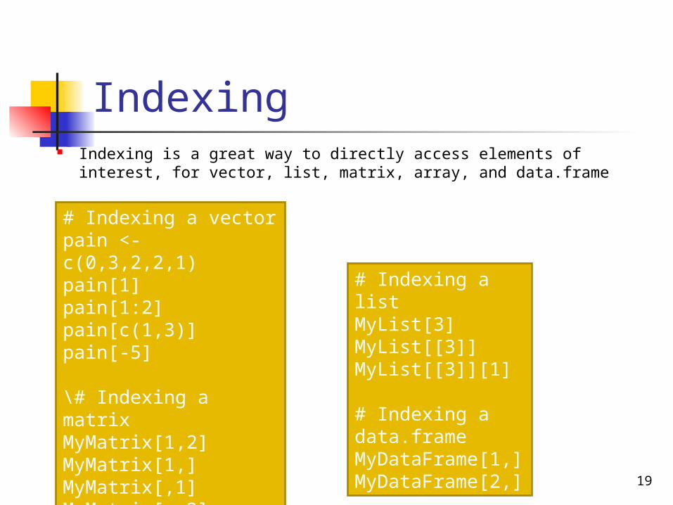
Indexing Indexing is a great way to directly access elements of
interest, for vector, list, matrix, array, and data.frame
# Indexing a vectorpain <- c(0,3,2,2,1)pain[1]pain[1:2]pain[c(1,3)]pain[-5]
\# Indexing a matrixMyMatrix[1,2]MyMatrix[1,]MyMatrix[,1]MyMatrix[,-2]
# Indexing a listMyList[3]MyList[[3]]MyList[[3]][1]
# Indexing a data.frameMyDataFrame[1,]MyDataFrame[2,]
112/04/18 20
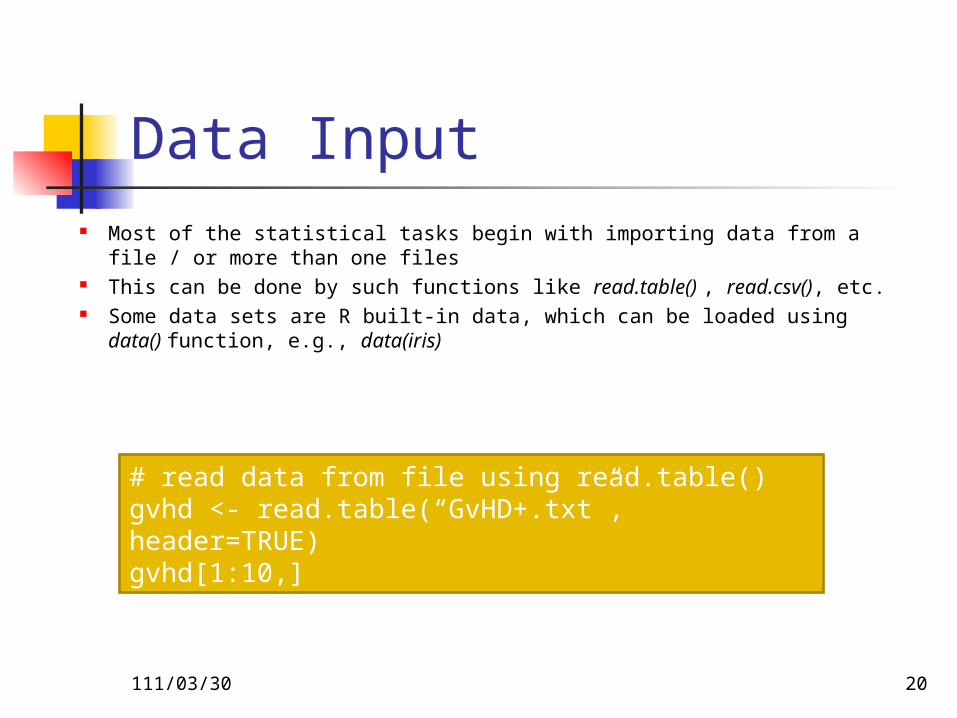
Data Input Most of the statistical tasks begin with importing data from a file / or
more than one files This can be done by such functions like read.table() , read.csv(), etc. Some data sets are R built-in data, which can be loaded using data()
function, e.g., data(iris)
# read data from file using read.table()gvhd <- read.table(“GvHD+.txt”, header=TRUE)gvhd[1:10,]
112/04/18 21
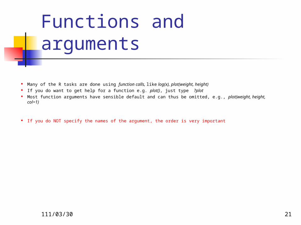
Functions and arguments
Many of the R tasks are done using function calls, like log(x), plot(weight, height) If you do want to get help for a function e.g. plot(), just type ?plot Most function arguments have sensible default and can thus be omitted, e.g., plot(weight, height, col=1)
If you do NOT specify the names of the argument, the order is very important
112/04/18 22
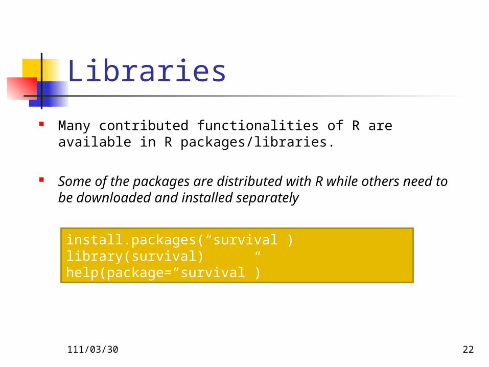
Libraries
Many contributed functionalities of R are available in R packages/libraries.
Some of the packages are distributed with R while others need to be downloaded and installed separately
install.packages(“survival”)library(survival)help(package=“survival”)
112/04/18 23
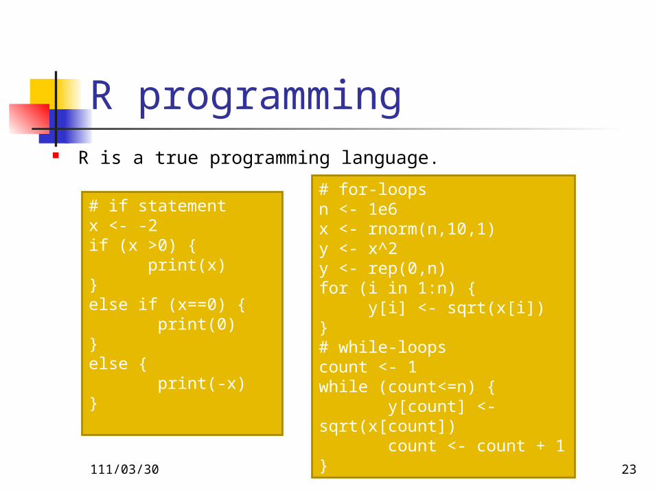
R programming R is a true programming language.
# if statementx <- -2if (x >0) { print(x)}else if (x==0) { print(0)}else { print(-x)}
# for-loopsn <- 1e6x <- rnorm(n,10,1)y <- x^2y <- rep(0,n)for (i in 1:n) { y[i] <- sqrt(x[i])}# while-loopscount <- 1 while (count<=n) { y[count] <- sqrt(x[count]) count <- count + 1}
112/04/18 24
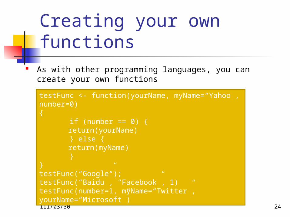
Creating your own functions
As with other programming languages, you can create your own functions
testFunc <- function(yourName, myName=“Yahoo”, number=0){ if (number == 0) {
return(yourName) } else {
return(myName) }}testFunc(“Google”);testFunc(“Baidu”, “Facebook”, 1)testFunc(number=1, myName=“Twitter”, yourName=“Microsoft”)
25
Outline
Why R, and R Paradigm References and links R Overview R Interface R Workspace Help R Packages Input/Output
26
Why R?
It's free! It runs on a variety of platforms including Wind
ows, Unix and MacOS. It provides an unparalleled platform for progra
mming new statistical methods in an easy and straightforward manner.
It contains advanced statistical routines not yet available in other packages.
It has state-of-the-art graphics capabilities.
27
R has a Steep Learning Curve (steeper for those that knew SAS or other software before)
First, while there are many introductory tutorials (covering data types, basic commands, the interface), none alone are comprehensive. In part, this is because much of the advanced functionality of R comes from hundreds of user contributed packages. Hunting for what you want can be time consuming, and it can be hard to get a clear overview of what procedures are available.
28
R has a Learning Curve(steeper for those that knew SAS or other software
before) The second reason is more transient. As users of statistical packages, we tend to run one controlled procedure for each type of analysis. Think of PROC GLM in SAS. We can carefully set up the run with all the parameters and options that we need. When we run the procedure, the resulting output may be a hundred pages long. We then sift through this output pulling out what we need and discarding the rest.
29
R paradigm is differentRather than setting up a complete analysis at once, the process is highly interactive. You run a command (say fit a model), take the results and process it through another command (say a set of diagnostic plots), take those results and process it through another command (say cross-validation), etc. The cycle may include transforming the data, and looping back through the whole process again. You stop when you feel that you have fully analyzed the data.
30
Web links Paul Geissler's excellent R tutorial Dave Robert's Excellent Labs on Ecological Analysis Excellent Tutorials by David Rossitier Excellent tutorial an nearly every aspect of R (c/o Rob Kabacoff) MOST
of these notes follow this web page format Introduction to R by Vincent Zoonekynd R Cookbook Data Manipulation Reference
31
Web links R time series tutorial R Concepts and Data Types
presentation by Deepayan Sarkar
Interpreting Output From lm() The R Wiki An Introduction to R Import / Export Manual R Reference Cards
32
Web links KickStart Hints on plotting data in R Regression and ANOVA Appendices to Fox Book on Regression JGR a Java-based GUI for R [Mac|Windows|Linux] A Handbook of Statistical Analyses Using R(Brian S. Everitt and Torsten Hothorn)
33
R OverviewR is a comprehensive statistical and graphical
programming language and is a dialect of the S language:
S: an interactive environment for data analysis developed at Bell Laboratories since 1976
1988 - S2: RA Becker, JM Chambers, A Wilks 1992 - S3: JM Chambers, TJ Hastie1998 - S4: JM Chambers
Exclusively licensed by AT&T/Lucent to Insightful Corporation, Seattle WA. Product name: “S-plus”. Implementation languages C, Fortran.R: initially written by Ross Ihaka and Robert Gentleman at Dep. of Statistics of U of Auckland, New Zealand during 1990s.
34
R Overview
You can enter commands one at a time at the command prompt (>) or run a set of commands from a source file.
There is a wide variety of data types, including vectors (numerical, character, logical), matrices, dataframes, and lists.
To quit R, use >q()
35
R Overview
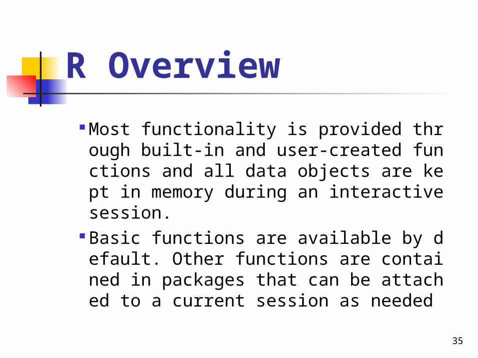
Most functionality is provided through built-in and user-created functions and all data objects are kept in memory during an interactive session.
Basic functions are available by default. Other functions are contained in packages that can be attached to a current session as needed
36
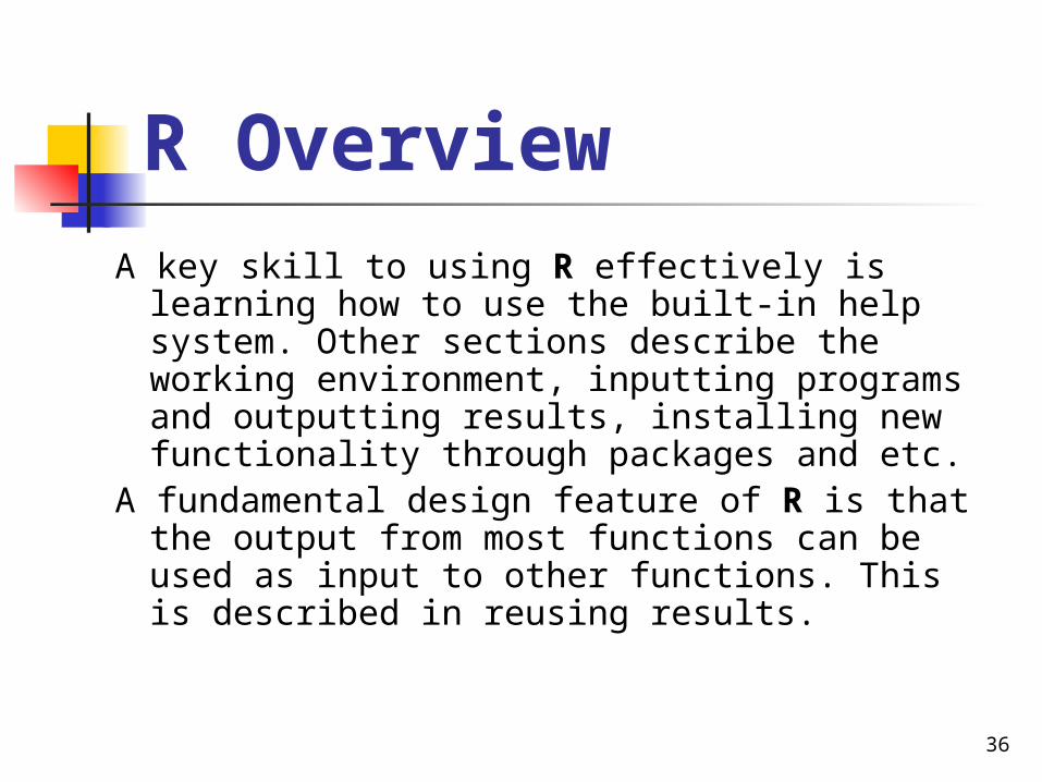
R OverviewA key skill to using R effectively is learning how to
use the built-in help system. Other sections describe the working environment, inputting programs and outputting results, installing new functionality through packages and etc.
A fundamental design feature of R is that the output from most functions can be used as input to other functions. This is described in reusing results.
37
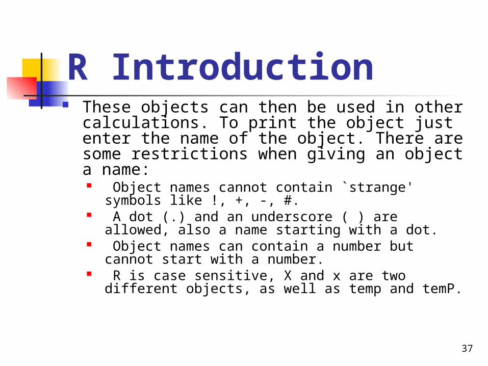
R Introduction These objects can then be used in other
calculations. To print the object just enter the name of the object. There are some restrictions when giving an object a name: Object names cannot contain `strange' symbols like
!, +, -, #. A dot (.) and an underscore ( ) are allowed, also a
name starting with a dot. Object names can contain a number but cannot
start with a number. R is case sensitive, X and x are two different
objects, as well as temp and temP.
38
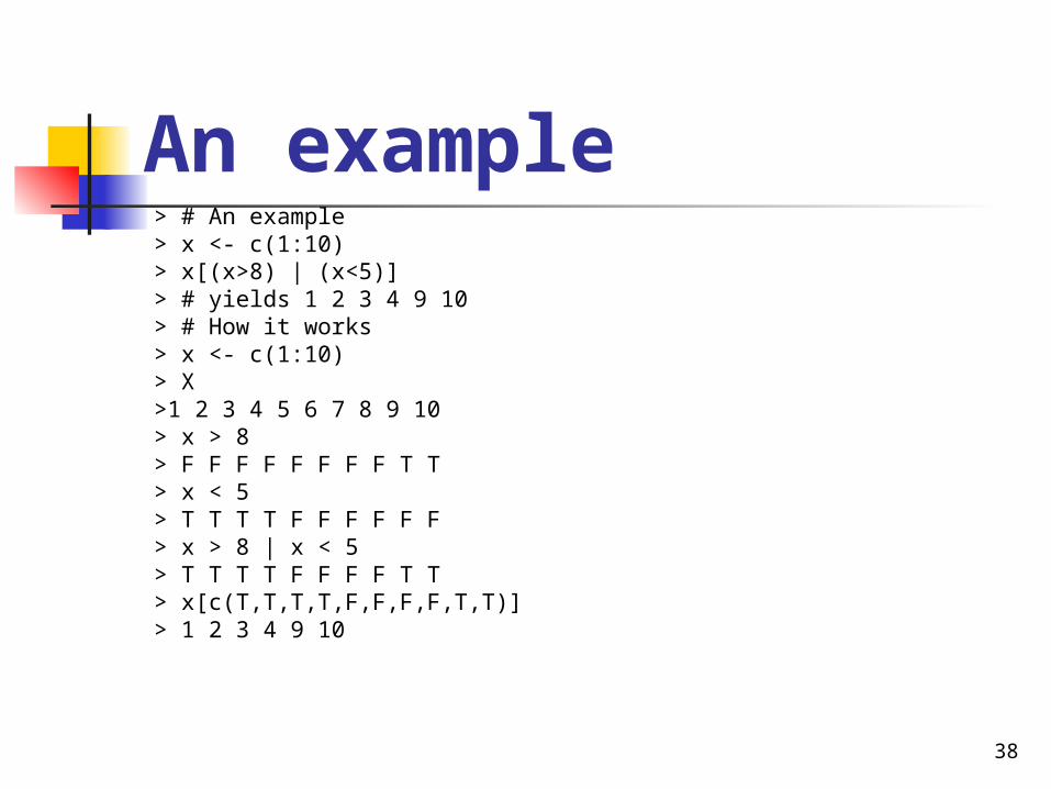
An example> # An example > x <- c(1:10)> x[(x>8) | (x<5)]> # yields 1 2 3 4 9 10> # How it works > x <- c(1:10)> X>1 2 3 4 5 6 7 8 9 10> x > 8> F F F F F F F F T T> x < 5> T T T T F F F F F F> x > 8 | x < 5> T T T T F F F F T T> x[c(T,T,T,T,F,F,F,F,T,T)]> 1 2 3 4 9 10
39
R Warning !
R is a case sensitive language. FOO, Foo, and foo are three different objects
40
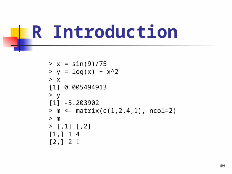
R Introduction
> x = sin(9)/75> y = log(x) + x^2> x[1] 0.005494913> y[1] -5.203902> m <- matrix(c(1,2,4,1), ncol=2)> m> [,1] [,2][1,] 1 4[2,] 2 1
41
R Workspace
Objects that you create during an R session are hold in memory, the collection of objects that you currently have is called the workspace. This workspace is not saved on disk unless you tell R to do so. This means that your objects are lost when you close R and not save the objects, or worse when R or your system crashes on you during a session.
42
R Workspace
When you close the RGui or the R console window, the system will ask if you want to save the workspace image. If you select to save the workspace image then all the objects in your current R session are saved in a file .RData. This is a binary file located in the working directory of R, which is by default the installation directory of R.
43
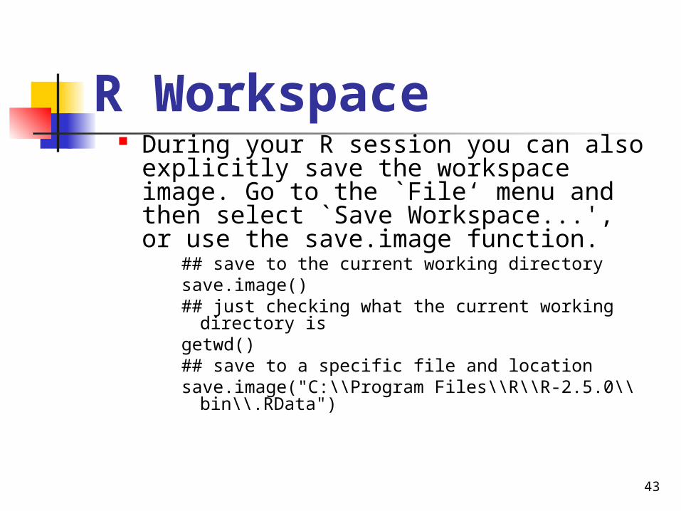
R Workspace During your R session you can also
explicitly save the workspace image. Go to the `File‘ menu and then select `Save Workspace...', or use the save.image function.
## save to the current working directorysave.image()## just checking what the current working
directory isgetwd()## save to a specific file and locationsave.image("C:\\Program Files\\R\\R-2.5.0\\
bin\\.RData")
Applied Statistical Computing and Graphics 44
R WorkspaceIf you have saved a workspace image
and you start R the next time, it will restore the workspace. So all your previously saved objects are available again. You can also explicitly load a saved workspace le, that could be the workspace image of someone else. Go the `File' menu and select `Load workspace...'.
Applied Statistical Computing and Graphics 45
R Workspace
Commands are entered interactively at the R user prompt. Up and down arrow keys scroll through your command history.
You will probably want to keep different projects in different physical directories.
Applied Statistical Computing and Graphics 46
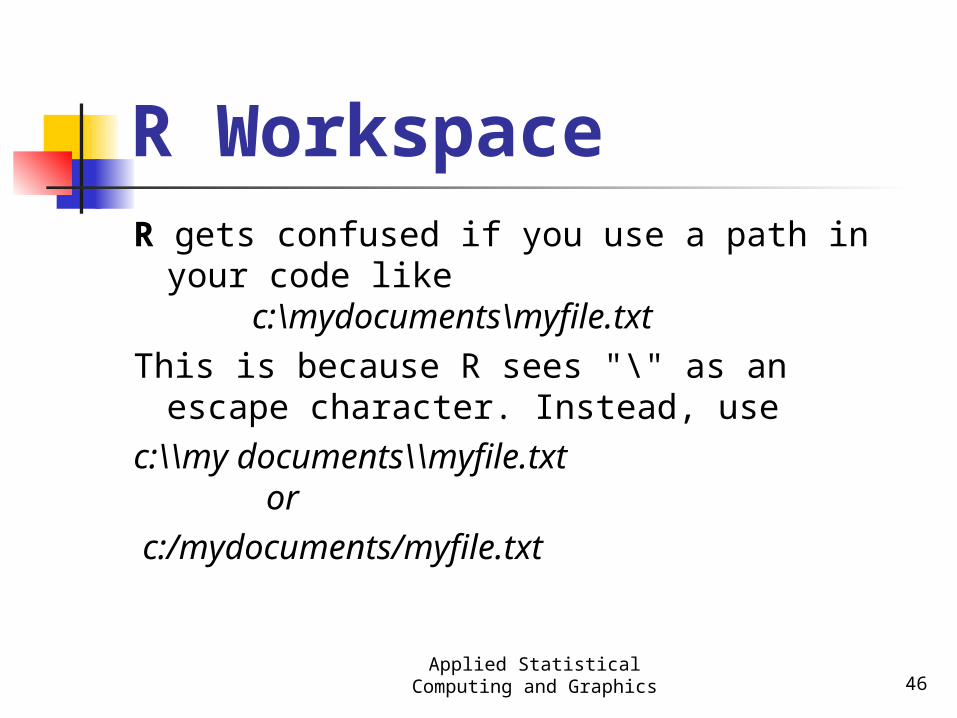
R WorkspaceR gets confused if you use a path in your
code like c:\mydocuments\myfile.txt
This is because R sees "\" as an escape character. Instead, use
c:\\my documents\\myfile.txt or
c:/mydocuments/myfile.txt
Applied Statistical Computing and Graphics 47
R Workspace
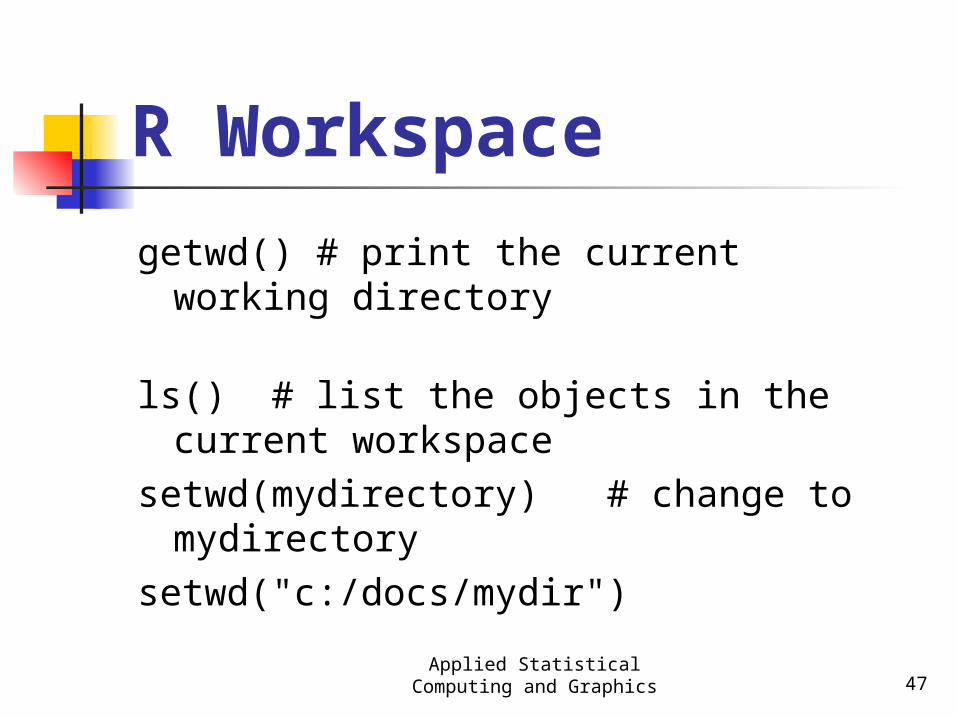
getwd() # print the current working directory
ls() # list the objects in the current workspace
setwd(mydirectory) # change to mydirectory
setwd("c:/docs/mydir")
48
R Workspace
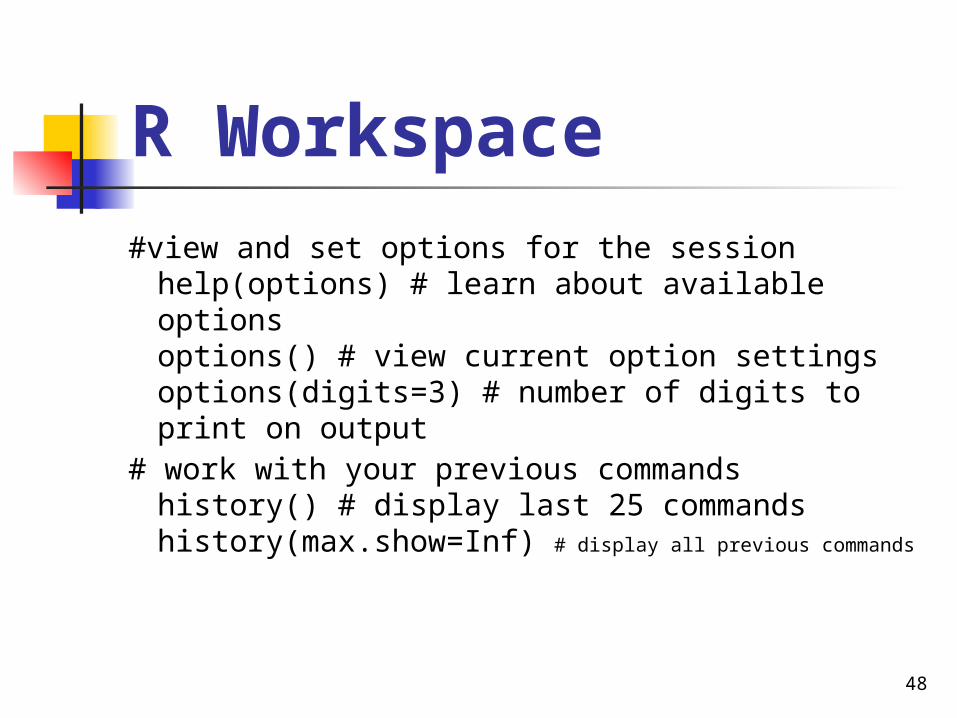
#view and set options for the sessionhelp(options) # learn about available optionsoptions() # view current option settingsoptions(digits=3) # number of digits to print on output
# work with your previous commandshistory() # display last 25 commandshistory(max.show=Inf) # display all previous commands
Applied Statistical Computing and Graphics 49
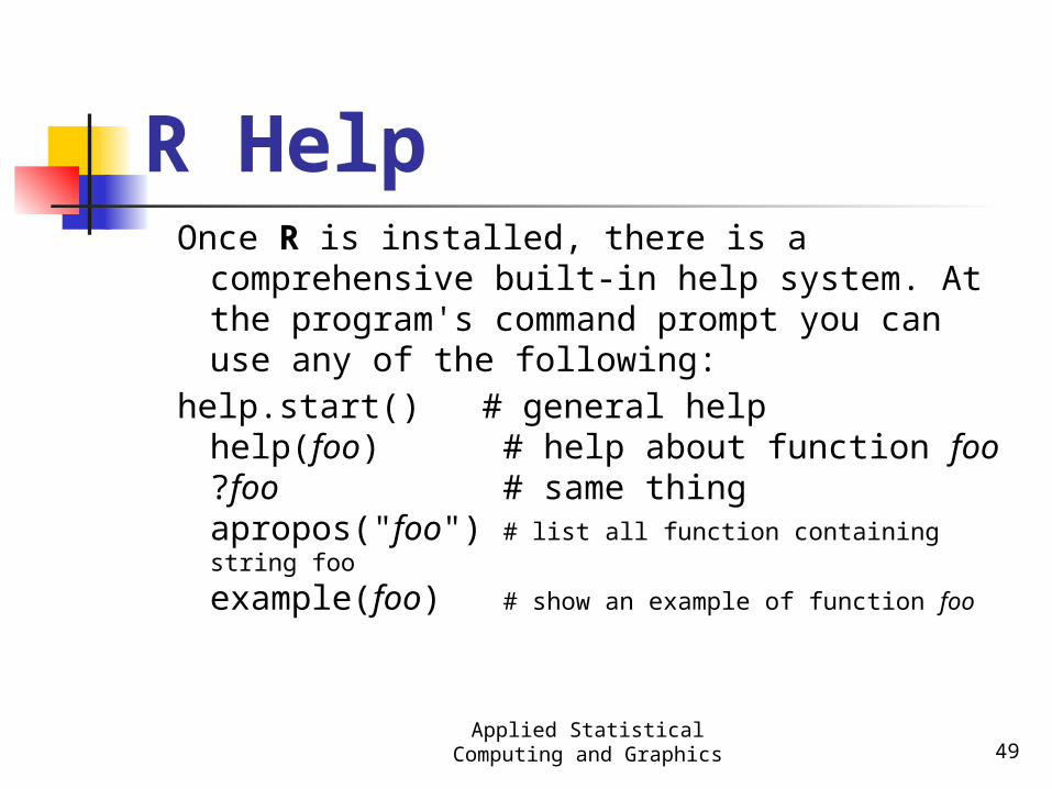
R HelpOnce R is installed, there is a
comprehensive built-in help system. At the program's command prompt you can use any of the following:
help.start() # general helphelp(foo) # help about function foo?foo # same thing apropos("foo") # list all function containing string foo
example(foo) # show an example of function foo
50
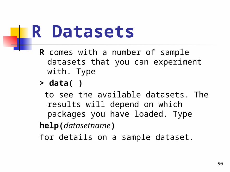
R DatasetsR comes with a number of sample
datasets that you can experiment with. Type
> data( ) to see the available datasets. The results
will depend on which packages you have loaded. Type
help(datasetname) for details on a sample dataset.
Applied Statistical Computing and Graphics 51
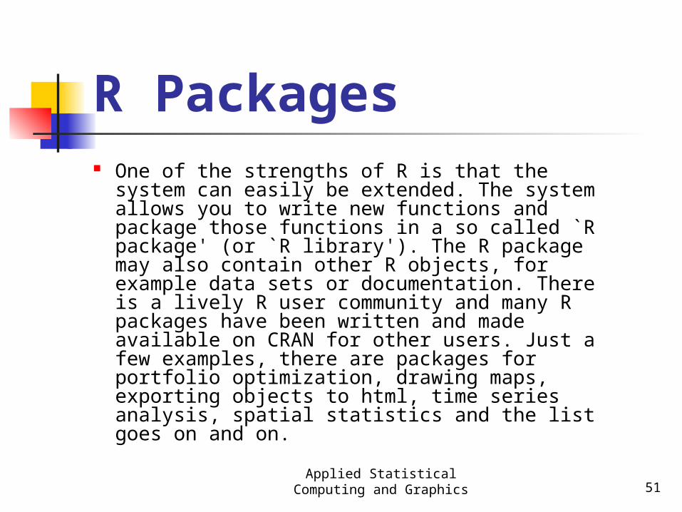
R Packages One of the strengths of R is that the system
can easily be extended. The system allows you to write new functions and package those functions in a so called `R package' (or `R library'). The R package may also contain other R objects, for example data sets or documentation. There is a lively R user community and many R packages have been written and made available on CRAN for other users. Just a few examples, there are packages for portfolio optimization, drawing maps, exporting objects to html, time series analysis, spatial statistics and the list goes on and on.
52
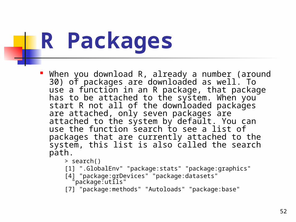
R Packages When you download R, already a number
(around 30) of packages are downloaded as well. To use a function in an R package, that package has to be attached to the system. When you start R not all of the downloaded packages are attached, only seven packages are attached to the system by default. You can use the function search to see a list of packages that are currently attached to the system, this list is also called the search path.
> search()[1] ".GlobalEnv" "package:stats" "package:graphics"[4] "package:grDevices" "package:datasets"
"package:utils"[7] "package:methods" "Autoloads" "package:base"
53
R Packages
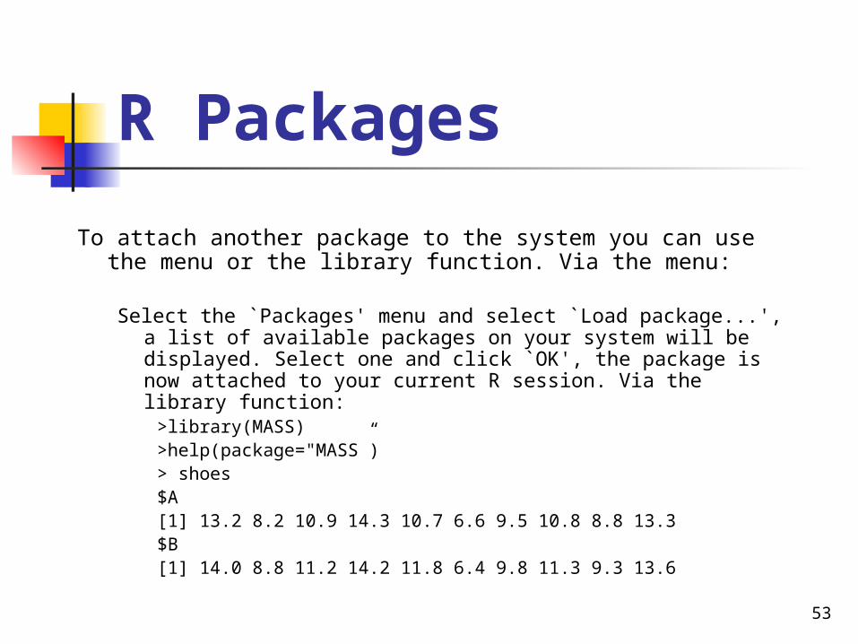
To attach another package to the system you can use the menu or the library function. Via the menu:
Select the `Packages' menu and select `Load package...', a list of available packages on your system will be displayed. Select one and click `OK', the package is now attached to your current R session. Via the library function:
>library(MASS)>help(package="MASS”)> shoes$A[1] 13.2 8.2 10.9 14.3 10.7 6.6 9.5 10.8 8.8 13.3$B[1] 14.0 8.8 11.2 14.2 11.8 6.4 9.8 11.3 9.3 13.6
Applied Statistical Computing and Graphics 54
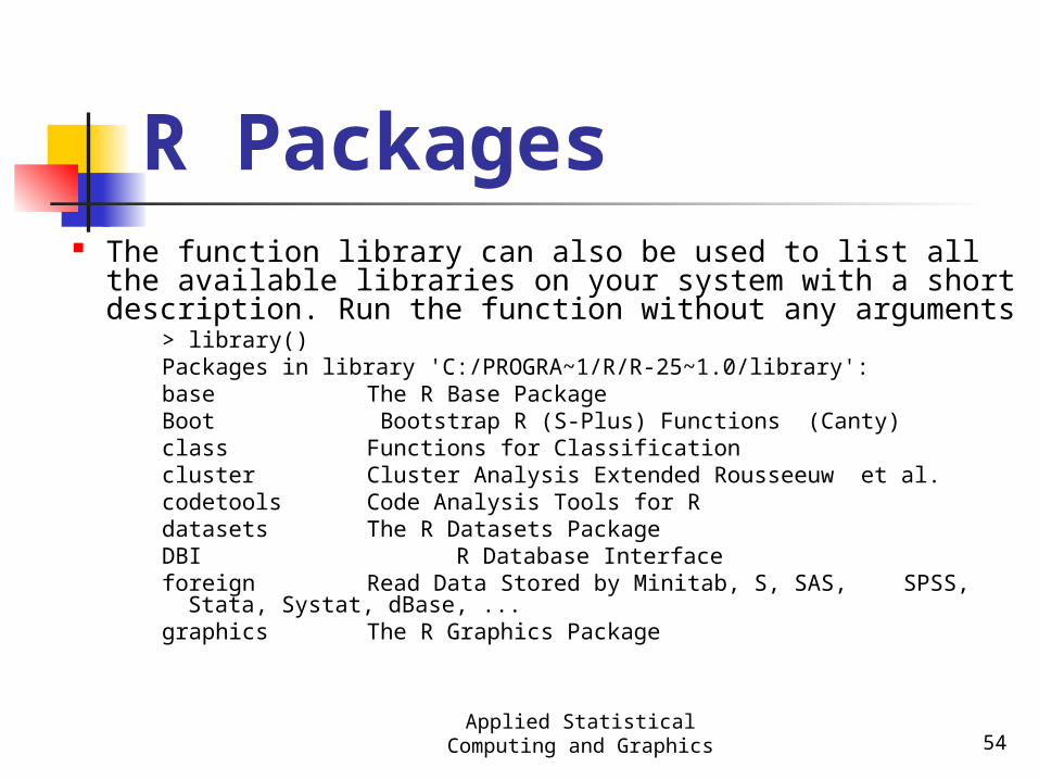
R Packages The function library can also be used to list all the
available libraries on your system with a short description. Run the function without any arguments
> library()Packages in library 'C:/PROGRA~1/R/R-25~1.0/library':base The R Base PackageBoot Bootstrap R (S-Plus) Functions (Canty)class Functions for Classificationcluster Cluster Analysis Extended Rousseeuw et al.codetools Code Analysis Tools for Rdatasets The R Datasets PackageDBI R Database Interfaceforeign Read Data Stored by Minitab, S, SAS,
SPSS, Stata, Systat, dBase, ...graphics The R Graphics Package
Applied Statistical Computing and Graphics 55
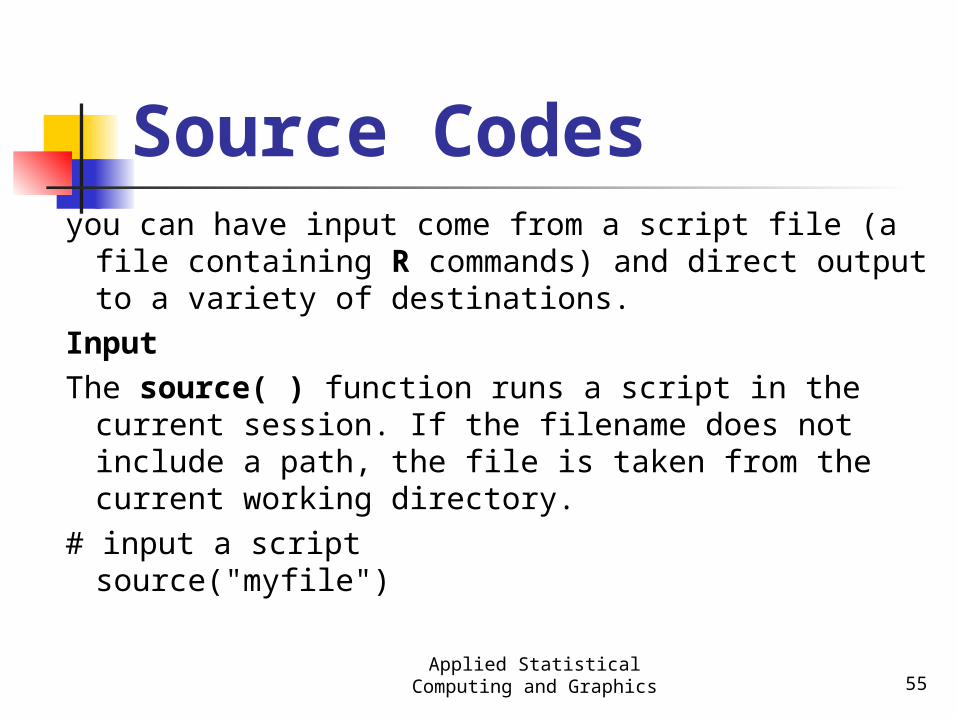
Source Codesyou can have input come from a script file (a file
containing R commands) and direct output to a variety of destinations.
Input The source( ) function runs a script in the current
session. If the filename does not include a path, the file is taken from the current working directory.
# input a scriptsource("myfile")
56
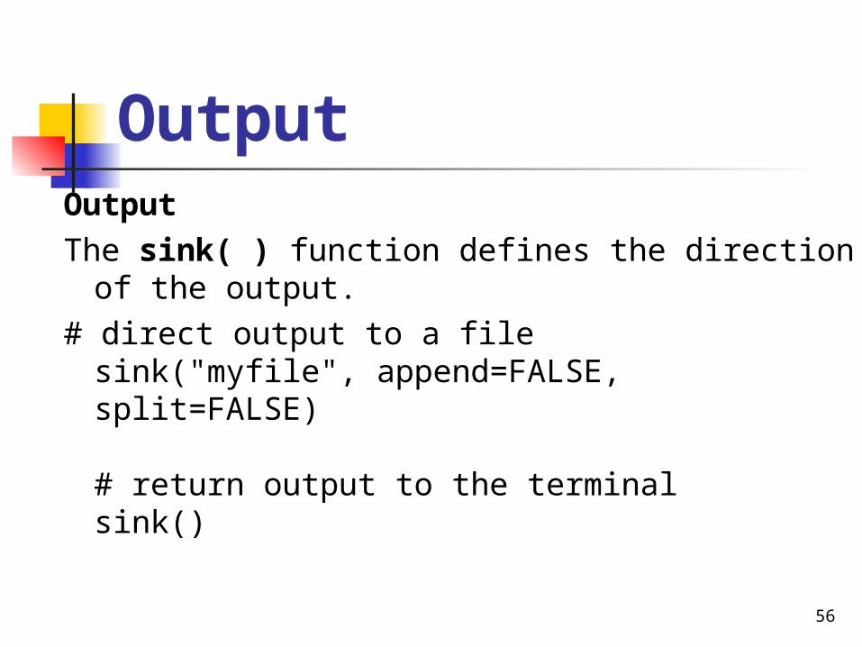
OutputOutputThe sink( ) function defines the direction of
the output. # direct output to a file
sink("myfile", append=FALSE, split=FALSE)
# return output to the terminal sink()
57
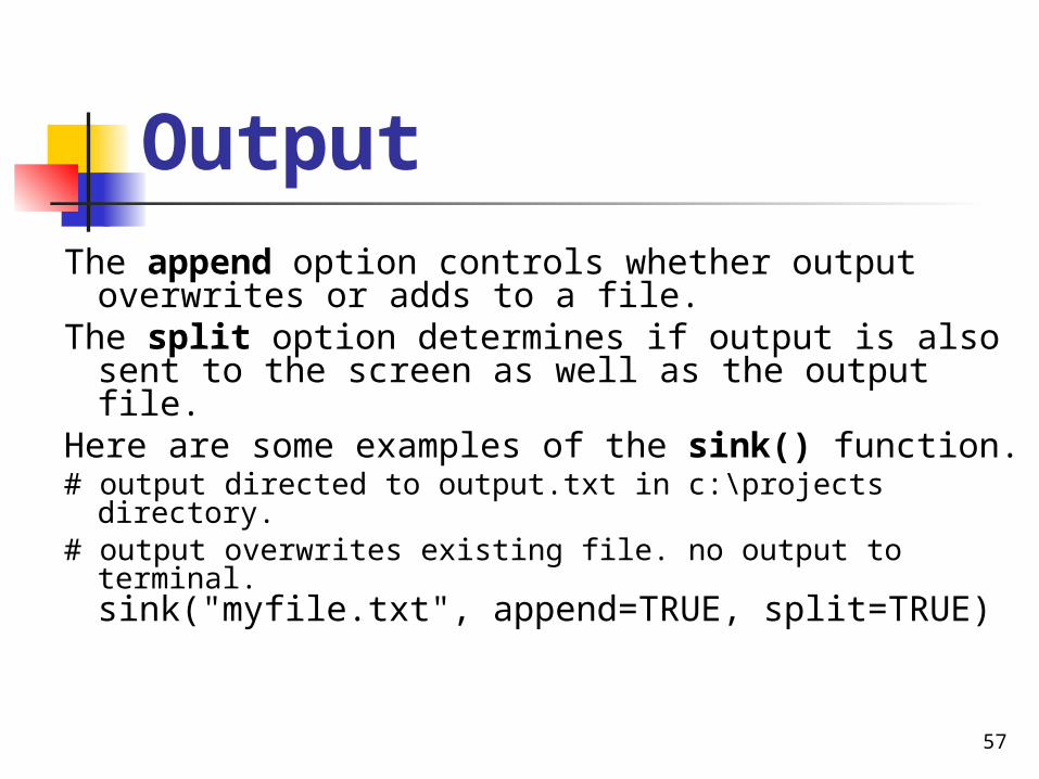
OutputThe append option controls whether output
overwrites or adds to a file.The split option determines if output is also
sent to the screen as well as the output file.Here are some examples of the sink()
function. # output directed to output.txt in c:\projects directory.# output overwrites existing file. no output to
terminal. sink("myfile.txt", append=TRUE, split=TRUE)
58
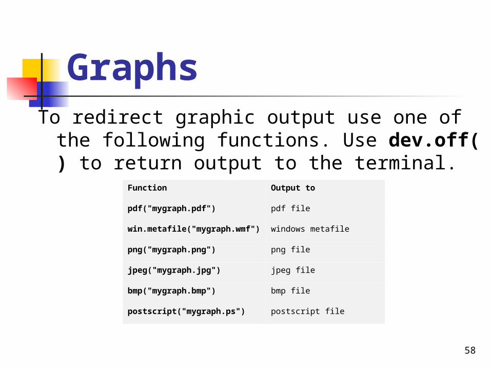
GraphsTo redirect graphic output use one of the
following functions. Use dev.off( ) to return output to the terminal.
Function Output to
pdf("mygraph.pdf") pdf file
win.metafile("mygraph.wmf") windows metafile
png("mygraph.png") png file
jpeg("mygraph.jpg") jpeg file
bmp("mygraph.bmp") bmp file
postscript("mygraph.ps") postscript file
59
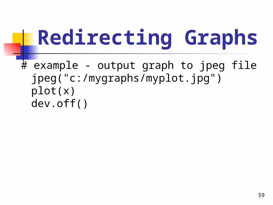
Redirecting Graphs# example - output graph to jpeg file
jpeg("c:/mygraphs/myplot.jpg")plot(x)dev.off()
60
Data input &output
Data Types Importing Data Keyboard Input Database Input Exporting Data Viewing Data
61
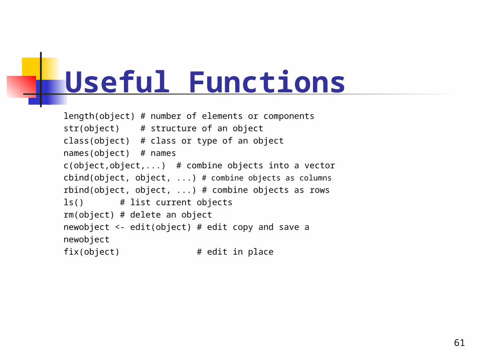
Useful Functionslength(object) # number of elements or componentsstr(object) # structure of an object class(object) # class or type of an objectnames(object) # namesc(object,object,...) # combine objects into a vectorcbind(object, object, ...) # combine objects as columns
rbind(object, object, ...) # combine objects as rows ls() # list current objectsrm(object) # delete an objectnewobject <- edit(object) # edit copy and save anewobject fix(object) # edit in place
62
From A Comma Delimited Text File
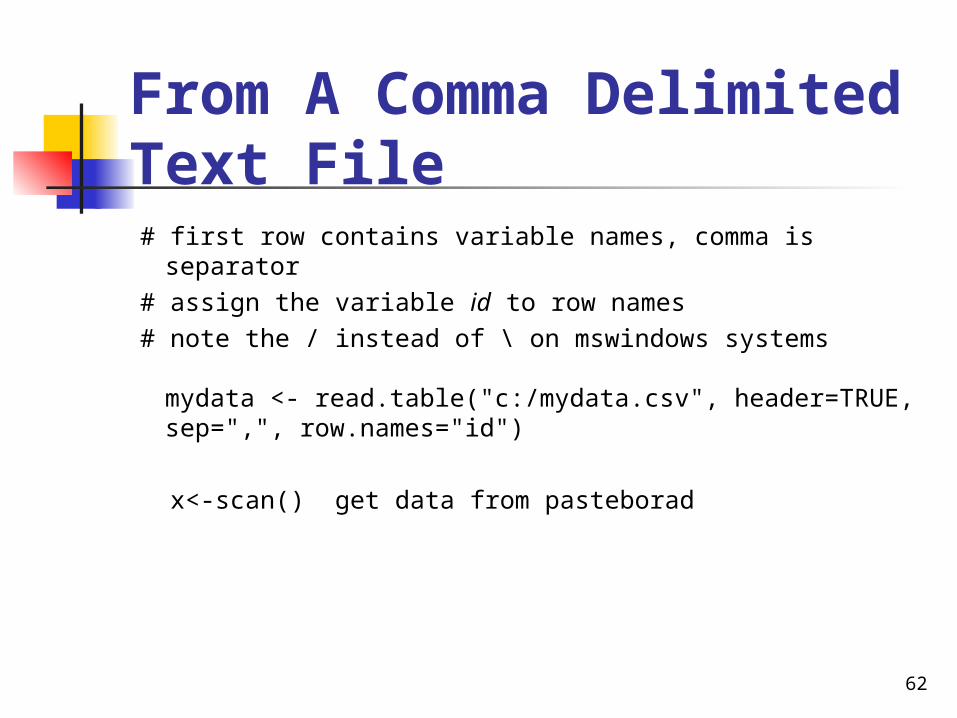
# first row contains variable names, comma is separator # assign the variable id to row names# note the / instead of \ on mswindows systems
mydata <- read.table("c:/mydata.csv", header=TRUE, sep=",", row.names="id")
x<-scan() get data from pasteborad
63
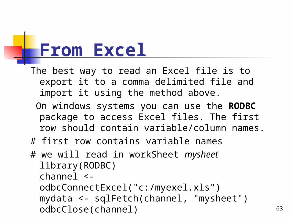
From ExcelThe best way to read an Excel file is to export it
to a comma delimited file and import it using the method above.
On windows systems you can use the RODBC package to access Excel files. The first row should contain variable/column names.
# first row contains variable names# we will read in workSheet mysheet
library(RODBC)channel <- odbcConnectExcel("c:/myexel.xls")mydata <- sqlFetch(channel, "mysheet")odbcClose(channel)
64
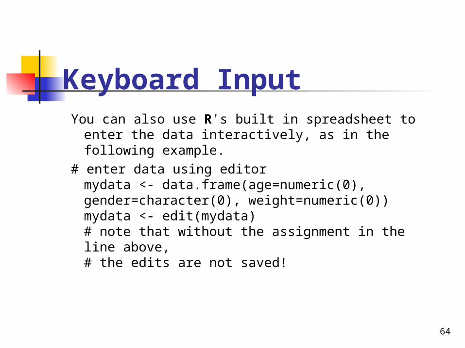
Keyboard Input You can also use R's built in spreadsheet to enter
the data interactively, as in the following example.
# enter data using editor mydata <- data.frame(age=numeric(0), gender=character(0), weight=numeric(0))mydata <- edit(mydata)# note that without the assignment in the line above, # the edits are not saved!
65
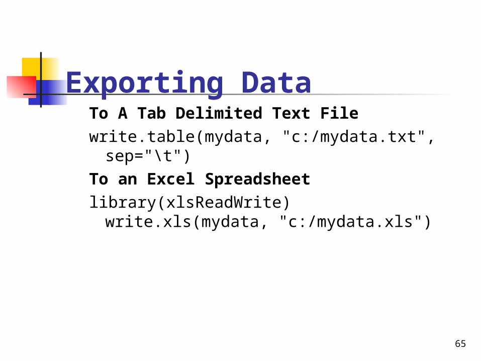
Exporting Data To A Tab Delimited Text Filewrite.table(mydata, "c:/mydata.txt", sep="\t") To an Excel Spreadsheet library(xlsReadWrite)
write.xls(mydata, "c:/mydata.xls")
66
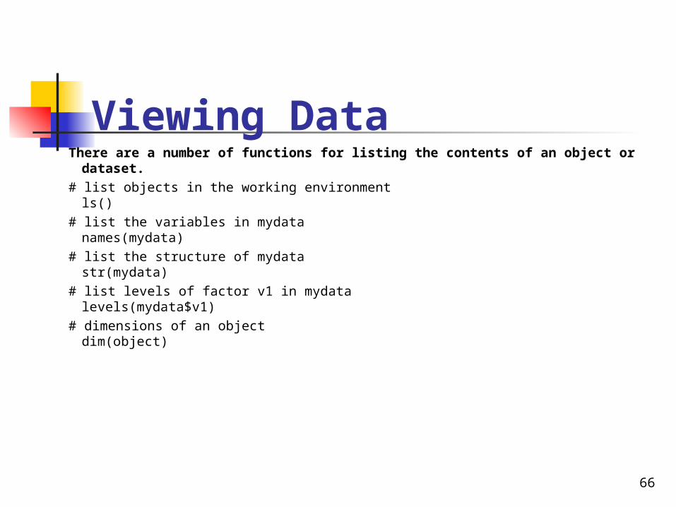
Viewing Data There are a number of functions for listing the contents of an object or
dataset. # list objects in the working environment
ls() # list the variables in mydata
names(mydata)# list the structure of mydata
str(mydata) # list levels of factor v1 in mydata
levels(mydata$v1)# dimensions of an object
dim(object)
Pactice
>data() AirPassengers ChickWeight
Practice in Biostatistics 67


![Dexterity and Functionality Enhancement of the SJTU ...rii.sjtu.edu.cn/images/a/a0/AIM2015.Xu.pdf · and meiwk1005]@sjtu.edu.cn). 25mm access port [8]. Picciagallo et al. constructed](https://static.documents.pub/doc/80x56/5a9995577f8b9a18628da34b/dexterity-and-functionality-enhancement-of-the-sjtu-riisjtueducnimagesaa0.jpg)