37
6.003: Signals and Systems Signals and Systems September 8, 2011 1
6.003: Signals and Systems
Signals and Systems
September 8, 2011 1

6.003: Signals and Systems Today’s handouts: Single package containing
• Slides for Lecture 1 • Subject Information & Calendar
Lecturer: Instructors:
TAs:
Denny Freeman Elfar Adalsteinsson
Russ Tedrake
Phillip Nadeau
Wenbang Xu
Website: mit.edu/6.003
Text: Signals and Systems – Oppenheim and Willsky
2

6.003: Homework
Doing the homework is essential for understanding the content. • where subject matter is/isn’t learned • equivalent to “practice” in sports or music
Weekly Homework Assignments • Conventional Homework Problems plus • Engineering Design Problems (Python/Matlab)
Open Office Hours ! • Stata Basement • Mondays and Tuesdays, afternoons and early evenings
3

6.003: Signals and Systems
Collaboration Policy • Discussion of concepts in homework is encouraged • Sharing of homework or code is not permitted and will be re
ported to the COD
Firm Deadlines • Homework must be submitted by the published due date • Each student can submit one late homework assignment without
penalty. • Grades on other late assignments will be multiplied by 0.5 (unless
excused by an Instructor, Dean, or Medical Official).
4
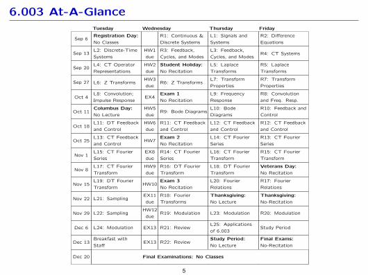
6.003 At-A-Glance
Sep 6Registration Day:
No Classes
R1: Continuous &
Discrete Systems
L1: Signals and
Systems
R2: Difference
Equations
Sep 13L2: Discrete-Time
Systems
HW1
due
R3: Feedback,
Cycles, and Modes
L3: Feedback,
Cycles, and ModesR4: CT Systems
Sep 20L4: CT Operator
Representations
HW2
due
Student Holiday:
No Recitation
L5: Laplace
Transforms
R5: Laplace
Transforms
Sep 27 L6: Z TransformsHW3
dueR6: Z Transforms
L7: Transform
Properties
R7: Transform
Properties
Oct 4L8: Convolution;
Impulse ResponseEX4
Exam 1
No Recitation
L9: Frequency
Response
R8: Convolution
and Freq. Resp.
Oct 11Columbus Day:
No Lecture
HW5
dueR9: Bode Diagrams
L10: Bode
Diagrams
R10: Feedback and
Control
Oct 18L11: DT Feedback
and Control
HW6
due
R11: CT Feedback
and Control
L12: CT Feedback
and Control
R12: CT Feedback
and Control
Oct 25L13: CT Feedback
and ControlHW7
Exam 2
No Recitation
L14: CT Fourier
Series
R13: CT Fourier
Series
Nov 1L15: CT Fourier
Series
EX8
due
R14: CT Fourier
Series
L16: CT Fourier
Transform
R15: CT Fourier
Transform
Nov 8L17: CT Fourier
Transform
HW9
due
R16: DT Fourier
Transform
L18: DT Fourier
Transform
Veterans Day:
No Recitation
Nov 15L19: DT Fourier
TransformHW10
Exam 3
No Recitation
L20: Fourier
Relations
R17: Fourier
Relations
Nov 22 L21: SamplingEX11
due
R18: Fourier
Transforms
Thanksgiving:
No Lecture
Thanksgiving:
No-Recitation
Nov 29 L22: SamplingHW12
dueR19: Modulation L23: Modulation R20: Modulation
Dec 6 L24: Modulation EX13 R21: ReviewL25: Applications
of 6.003Study Period
Dec 13Breakfast with
StaffEX13 R22: Review
Study Period:
No Lecture
Final Exams:
No-Recitation
Dec 20 finals finals finals finals finals
Tuesday Wednesday Thursday Friday
Final Examinations: No Classes
5

6.003: Signals and Systems
Weekly meetings with class representatives • help staff understand student perspective • learn about teaching
Tentatively meet on Thursday afternoon
Interested? ...
6

The Signals and Systems Abstraction
Describe a system (physical, mathematical, or computational) by the way it transforms an input signal into an output signal.
systemsignal
in
signal
out
7

Example: Mass and Spring
x(t)
y(t)
mass &springsystem
x(t) y(t)
t t
8

Example: Tanks
r0(t)
r1(t)
r2(t)
h1(t)
h2(t)
tanksystem
r0(t) r2(t)
t t
9

Example: Cell Phone System
sound in
sound out
cellphonesystem
sound in sound out
t t
10

Signals and Systems: Widely Applicable
The Signals and Systems approach has broad application: electrical, mechanical, optical, acoustic, biological, financial, ...
mass &springsystem
x(t) y(t)
t t
r0(t)
r1(t)
r2(t)
h1(t)
h2(t) tanksystem
r0(t) r2(t)
t t
cellphonesystem
sound in sound out
t t
11

Signals and Systems: Modular
The representation does not depend upon the physical substrate.
sound in
sound out
cellphone
tower towercell
phonesound
in
E/M optic
fiber
E/M soundout
focuses on the flow of information, abstracts away everything else 12

Signals and Systems: Hierarchical
Representations of component systems are easily combined.
Example: cascade of component systems
cellphone
tower towercell
phonesound
in
E/M optic
fiber
E/M soundout
Composite system
cell phone systemsound
insound
out
Component and composite systems have the same form, and are analyzed with same methods.
13

Signals and Systems
Signals are mathematical functions. • independent variable = time • dependent variable = voltage, flow rate, sound pressure
mass &springsystem
x(t) y(t)
t t
tanksystem
r0(t) r2(t)
t t
cellphonesystem
sound in sound out
t t
14

Signals and Systems
continuous “time” (CT) and discrete “time” (DT)
t
x(t)
0 2 4 6 8 10n
x[n]
0 2 4 6 8 10
Signals from physical systems often functions of continuous time. • mass and spring • leaky tank
Signals from computation systems often functions of discrete time. • state machines: given the current input and current state, what
is the next output and next state. 15

Signals and Systems
Sampling: converting CT signals to DT
t
x(t)
0T 2T 4T 6T 8T 10Tn
x[n] = x(nT )
0 2 4 6 8 10
T = sampling interval
Important for computational manipulation of physical data. • digital representations of audio signals (e.g., MP3) • digital representations of images (e.g., JPEG)
16

Signals and Systems
Reconstruction: converting DT signals to CT
zero-order hold
n
x[n]
0 2 4 6 8 10t
x(t)
0 2T 4T 6T 8T 10T
T = sampling interval
commonly used in audio output devices such as CD players 17
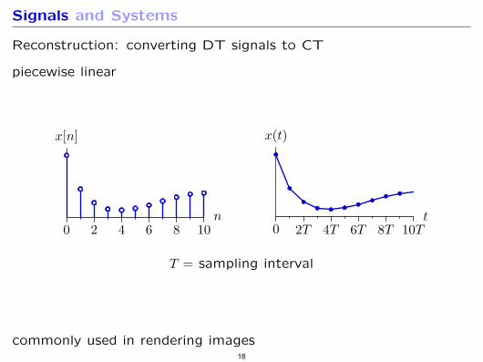
Signals and Systems
Reconstruction: converting DT signals to CT
piecewise linear
n
x[n]
0 2 4 6 8 10t
x(t)
0 2T 4T 6T 8T 10T
T = sampling interval
commonly used in rendering images 18

Check Yourself
Computer generated speech (by Robert Donovan)
t
f(t)
Listen to the following four manipulated signals: f1(t), f2(t), f3(t), f4(t).
How many of the following relations are true?
• f1(t) = f(2t) • f2(t) = −f(t) • f3(t) = f(2t) • f4(t) = 1
3 f(t)
19

Check Yourself
Computer generated speech (by Robert Donovan)
t
f(t)
Listen to the following four manipulated signals: f1(t), f2(t), f3(t), f4(t).
How many of the following relations are true? 2
• f1(t) = f(2t) √
• f2(t) = −f(t) X • f3(t) = f(2t) X • f4(t) = 1
3 f(t) √
20
−250 0 250
−25
00
250
y
x
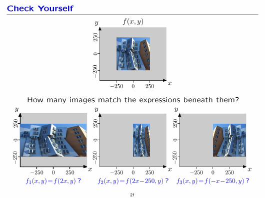
f1(x, y)=f(2x, y) ?−250 0 250
−25
00
250
y
x
f2(x, y)=f(2x−250, y) ?−250 0 250
−25
00
250
y
x
f3(x, y)=f(−x−250, y) ?
−250 0 250−
250
025
0
y
x
f(x, y)
How many images match the expressions beneath them?
Check Yourself
21

−250 0 250
−25
00
250
y
x
f(x, y)−250 0 250
−25
00
250
y
x
f1(x, y) = f(2x, y) ?−250 0 250
−25
00
250
y
x
f2(x, y) = f(2x−250, y) ?−250 0 250
−25
00
250
y
x
f3(x, y) = f(−x−250, y) ?
Check Yourself
√ x = 0 → f1(0, y) = f(0, y) x = 250 → f1(250, y) = f(500, y) X
√ x = 0 → f2(0, y) = f(−250, y) √ x = 250 → f2(250, y) = f(250, y)
x = 0 → f3(0, y) = f(−250, y) X x = 250 → f3(250, y) = f(−500, y) X
22
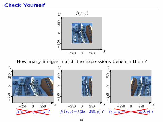
−250 0 250
−25
00
250
y
x
f1(x, y)=f(2x, y) ?−250 0 250
−25
00
250
y
x
f2(x, y)=f(2x−250, y) ?−250 0 250
−25
00
250
y
x
f3(x, y)=f(−x−250, y) ?
−250 0 250−
250
025
0
y
x
f(x, y)
How many images match the expressions beneath them?
Check Yourself
23
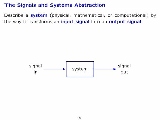
The Signals and Systems Abstraction
Describe a system (physical, mathematical, or computational) by the way it transforms an input signal into an output signal.
systemsignal
in
signal
out
24
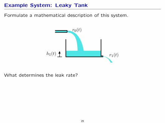
Example System: Leaky Tank
Formulate a mathematical description of this system.
What determines the leak rate?
r0(t)
r1(t)h1(t)
25
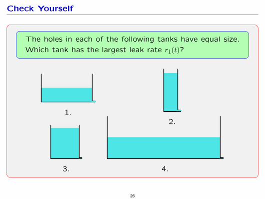
Check Yourself
The holes in each of the following tanks have equal size. Which tank has the largest leak rate r1(t)?
3. 4.
1.2.
26

Check Yourself
The holes in each of the following tanks have equal size. Which tank has the largest leak rate r1(t)? 2
3. 4.
1.2.
27
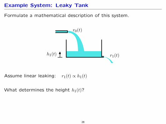
Example System: Leaky Tank
Formulate a mathematical description of this system.
r0(t)
r1(t)h1(t)
Assume linear leaking: r1(t) ∝ h1(t)
What determines the height h1(t)?
28

Example System: Leaky Tank
Formulate a mathematical description of this system.
r0(t)
r1(t)h1(t)
Assume linear leaking: r1(t) ∝ h1(t)
dh1(t)Assume water is conserved: ∝ r0(t) − r1(t)
dt
dr1(t)Solve: ∝ r0(t) − r1(t)
dt
29

Check Yourself
What are the dimensions of constant of proportionality C?
dr1(t) dt
= C �
r0(t) − r1(t) �
30
� �
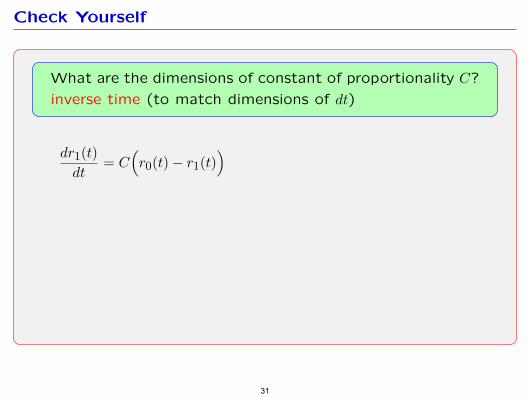
Check Yourself
What are the dimensions of constant of proportionality C? inverse time (to match dimensions of dt)
dr1(t) dt
= C r0(t) − r1(t)
31
( )

Analysis of the Leaky Tank
Call the constant of proportionality 1/τ .
Then τ is called the time constant of the system.
dr1(t) r0(t) r1(t)= − dt τ τ
32

Check Yourself
Which tank has the largest time constant τ?
3. 4.
1.2.
33
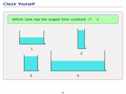
Check Yourself
Which tank has the largest time constant τ? 4
3. 4.
1.2.
34
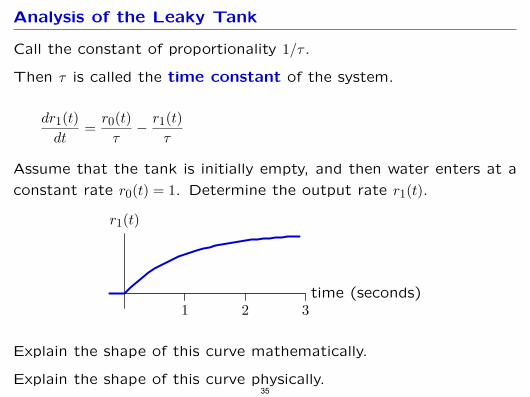
Analysis of the Leaky Tank
Call the constant of proportionality 1/τ .
Then τ is called the time constant of the system.
dr1(t) r0(t) r1(t)= − dt τ τ
Assume that the tank is initially empty, and then water enters at a constant rate r0(t) = 1. Determine the output rate r1(t).
time (seconds)
r1(t)
1 2 3
Explain the shape of this curve mathematically.
Explain the shape of this curve physically. 35

Leaky Tanks and Capacitors
Although derived for a leaky tank, this sort of model can be used to represent a variety of physical systems.
Water accumulates in a leaky tank.
r0(t)
r1(t)h1(t)
Charge accumulates in a capacitor.
C v
+
−
ii io
dv dt
= ii − io
C ∝ ii − io analogous to
dh dt
∝ r0 − r1 36

MIT OpenCourseWare http://ocw.mit.edu
6.003 Signals and Systems Fall 2011
For information about citing these materials or our Terms of Use, visit: http://ocw.mit.edu/terms.


