Lecture 10: Endogenous Growth

ECO 503: Macroeconomic Theory I

Benjamin Moll

Princeton University

Fall 2014

1 / 45

Plan of Lecture

• Last time: sustained long-run growth with exogenousproductivity growth

• This time: sustained long-run growth from purelyendogenous sources

2 / 45

Plan of Lecture

1 Simplest possible endogenous growth model: AK model

2 Endogenous growth from human capital accumulation:Lucas (1988), “On the Mechanics of Economic Development”

3 If time (i.e. probably not):Romer (1990), “Endogenous Technological Change”

3 / 45

AK model• Originally due to Romer (1986), Rebelo (1991), also seeAcemoglu Ch. 11

• Consider standard growth model

• Preferences:∫ ∞

0e−ρt c(t)

1−σ − 1

1− σ

• Technology:

y = F (k , h), c + i = y , k = i − δk

• Endowments: one units of time, k(0) = k0.

• Add one little twist: “AK production function”

F (k , h) = Ak

• e.g. Cobb-Douglas y = Akαh1−α with α = 1.

• Note: usual Inada condition limk→∞ f ′(k) = 0 is no longersatisfied. Instead

′4 / 45

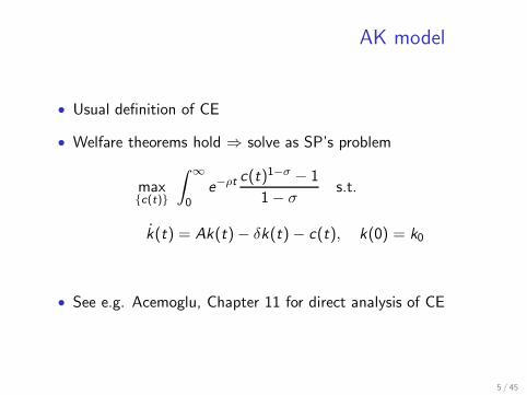
AK model

• Usual definition of CE

• Welfare theorems hold ⇒ solve as SP’s problem

max{c(t)}

∫ ∞

0e−ρt c(t)

1−σ − 1

1− σs.t.

k(t) = Ak(t)− δk(t)− c(t), k(0) = k0

• See e.g. Acemoglu, Chapter 11 for direct analysis of CE

5 / 45

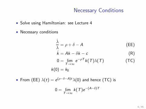
Necessary Conditions

• Solve using Hamiltonian: see Lecture 4

• Necessary conditions

λ

λ= ρ+ δ − A (EE)

k = Ak − δk − c (R)

0 = limT→∞

e−ρT k(T )λ(T ) (TC)

k(0) = k0

• From (EE) λ(t) = e(ρ−δ−A)tλ(0) and hence (TC) is

0 = limT→∞

k(T )e−(A−δ)T

6 / 45

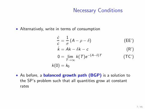
Necessary Conditions

• Alternatively, write in terms of consumption

c

c=

1

σ(A− ρ− δ) (EE’)

k = Ak − δk − c (R’)

0 = limT→∞

k(T )e−(A−δ)T (TC’)

k(0) = k0

• As before, a balanced growth path (BGP) is a solution tothe SP’s problem such that all quantities grow at constantrates

7 / 45

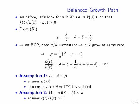
Balanced Growth Path• As before, let’s look for a BGP, i.e. a k(0) such thatk(t)/k(t) = g , t ≥ 0

• From (R’)

g =k

k= A− δ −

c

k• ⇒ on BGP, need c/k =constant ⇒ c , k grow at same rate

⇒ g =1

σ(A− ρ− δ)

c(t)

k(t)= A− δ −

1

σ(A− ρ− δ), ∀t

• Assumption 1: A− δ > ρ• ensures g > 0

• also ensures A > δ ⇒ (TC’) is satisfied

• Assumption 2: (1− σ)(A− δ) < ρ• ensures c(t)/k(t) > 0

8 / 45

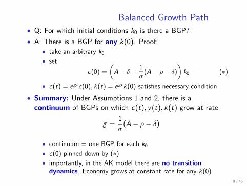
Balanced Growth Path• Q: For which initial conditions k0 is there a BGP?

• A: There is a BGP for any k(0). Proof:

• take an arbitrary k0

• set

c(0) =

(

A− δ −1

σ(A− ρ− δ)

)

k0 (∗)

• c(t) = egtc(0), k(t) = egtk(0) satisfies necessary condition

• Summary: Under Assumptions 1 and 2, there is acontinuum of BGPs on which c(t), y(t), k(t) grow at rate

g =1

σ(A − ρ− δ)

• continuum = one BGP for each k0

• c(0) pinned down by (∗)

• importantly, in the AK model there are no transitiondynamics. Economy grows at constant rate for any k(0)

9 / 45

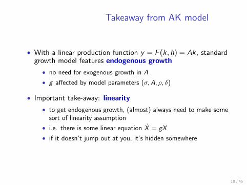
Takeaway from AK model

• With a linear production function y = F (k , h) = Ak , standardgrowth model features endogenous growth

• no need for exogenous growth in A

• g affected by model parameters (σ,A, ρ, δ)

• Important take-away: linearity

• to get endogenous growth, (almost) always need to make somesort of linearity assumption

• i.e. there is some linear equation X = gX

• if it doesn’t jump out at you, it’s hidden somewhere

10 / 45

Lucas (1988): “On the Mechanics of

Economic Development”

• One of most cited papers in economicshttps://ideas.repec.org/top/top.item.nbcites.html

• Famous quote (p.5):

• “I do not see how one can look at figures like these without

seeing them representing possibilities. Is there some action a

government of India could take that would lead the Indian

economy to grow like Indonesia’s or Egypt’s? If so, what

exactly? If not, what is it about the ”nature of India” that

makes it so? The consequences for human welfare involved in

questions like these are simply staggering: once one starts tothink about them, it is hard to think about anythingelse.”

11 / 45

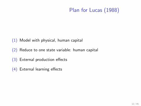
Plan for Lucas (1988)

(1) Model with physical, human capital

(2) Reduce to one state variable: human capital

(3) External production effects

(4) External learning effects

12 / 45

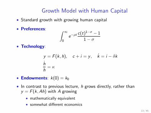
Growth Model with Human Capital

• Standard growth with growing human capital

• Preferences:∫ ∞

0e−ρt c(t)

1−σ − 1

1− σ

• Technology:

y = F (k , h), c + i = y , k = i − δk

h

h= κ

• Endowments: k(0) = k0

• In contrast to previous lecture, h grows directly, rather thany = F (k ,Ah) with A growing

• mathematically equivalent

• somewhat different economics

13 / 45

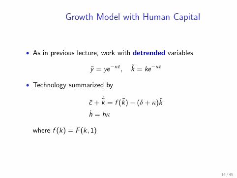
Growth Model with Human Capital

• As in previous lecture, work with detrended variables

y = ye−κt , k = ke−κt

• Technology summarized by

c + ˙k = f (k)− (δ + κ)k

h = hκ

where f (k) = F (k , 1)

14 / 45

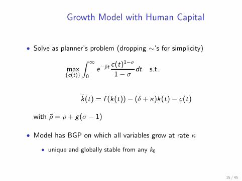
Growth Model with Human Capital

• Solve as planner’s problem (dropping ∼’s for simplicity)

max{c(t)}

∫ ∞

0e−ρt c(t)

1−σ

1− σdt s.t.

k(t) = f (k(t))− (δ + κ)k(t)− c(t)

with ρ = ρ+ g(σ − 1)

• Model has BGP on which all variables grow at rate κ

• unique and globally stable from any k0

15 / 45

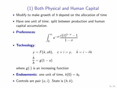
(1) Both Physical and Human Capital

• Modify to make growth of h depend on the allocation of time

• Have one unit of time: split between production and humancapital accumulation.

• Preferences:∫ ∞

0e−ρt c(t)

1−σ − 1

1− σ

• Technology:

y = F (k , uh), c + i = y , k = i − δk

h

h= g(1 − u)

where g(·) is an increasing function

• Endowments: one unit of time, k(0) = k0

• Controls are pair (u, i). State is (h, k).

16 / 45

Both Physical and Human Capital

• For best complete development, see

• Caballe and Santos, JPE, 1993

For earlier versions, see

• Uzawa, 1965, IER

• Razin, 1972, REStud

• Lucas, 1988, JME

• Rebelo, 1990, JPE

17 / 45

(2) Model with Human Capital Only

• Interesting, but complicated literature.

• And want to add further complication of external effects.

• Reduce to one state variable by dropping physical capital.

• An “Ak” model – for us, “Ah”

18 / 45

Model with Human Capital Only

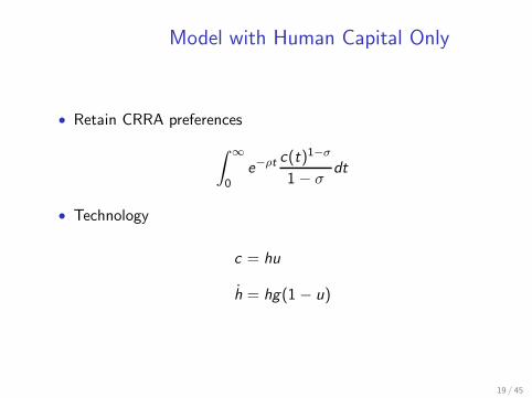
• Retain CRRA preferences

∫ ∞

0e−ρt c(t)

1−σ

1− σdt

• Technology

c = hu

h = hg(1 − u)

19 / 45

Model with Human Capital Only

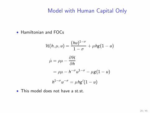
• Hamiltonian and FOCs

H(h, µ, u) =(hu)1−σ

1− σ+ µhg(1− u)

µ = ρµ−∂H

∂h

= ρµ− h−σu1−σ − µg(1− u)

h1−σu−σ = µhg ′(1− u)

• This model does not have a st.st.

20 / 45

Balanced Growth Path (BGP)

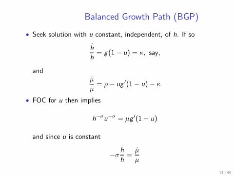
• Seek solution with u constant, independent, of h. If so

h

h= g(1− u) = κ, say,

andµ

µ= ρ− ug ′(1− u)− κ

• FOC for u then implies

h−σu−σ = µg ′(1− u)

and since u is constant

−σh

h=

µ

µ

21 / 45

BGP

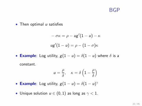
• Then optimal u satisfies

− σκ = ρ− ug ′(1− u)− κ

ug ′(1− u) = ρ− (1− σ)κ

• Example: Log utility, g(1 − u) = δ(1 − u) where δ is a

constant.

u =ρ

δ, κ = δ

(

1−ρ

δ

)

• Example: Log utility, g(1 − u) = δ(1 − u)γ

• Unique solution u ∈ (0, 1) as long as γ < 1.

22 / 45

(3),(4) Externalities

• Many people argue: important feature of human capital =externalities

• Here: two versions

• external production effect

• external learning effect

• Also useful tool: solving models with externalities

• externalities ⇒ welfare theorems fail

• here: trick so that can still solve CE with externalities asplanning problem

• “(k ,K ) models”. Here: “(h,H) model”

• same trick also applies in other cases, e.g. models withexternalities

23 / 45

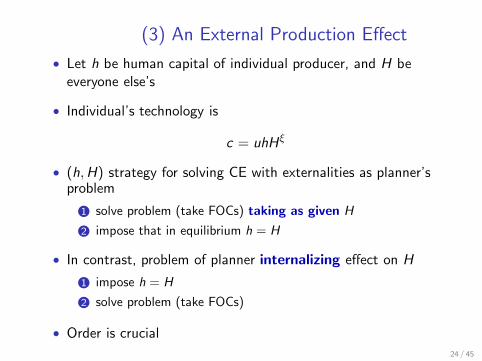
(3) An External Production Effect

• Let h be human capital of individual producer, and H beeveryone else’s

• Individual’s technology is

c = uhHξ

• (h,H) strategy for solving CE with externalities as planner’sproblem

1 solve problem (take FOCs) taking as given H

2 impose that in equilibrium h = H

• In contrast, problem of planner internalizing effect on H

1 impose h = H

2 solve problem (take FOCs)

• Order is crucial

24 / 45

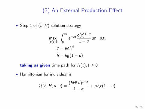
(3) An External Production Effect

• Step 1 of (h,H) solution strategy

max{u(t)}

∫ ∞

0e−ρt c(t)

1−σ

1− σdt s.t.

c = uhHξ

h = hg(1 − u)

taking as given time path for H(t), t ≥ 0

• Hamiltonian for individual is

H(h,H, µ, u) =(hHξu)1−σ

1− σ+ µhg(1− u)

25 / 45

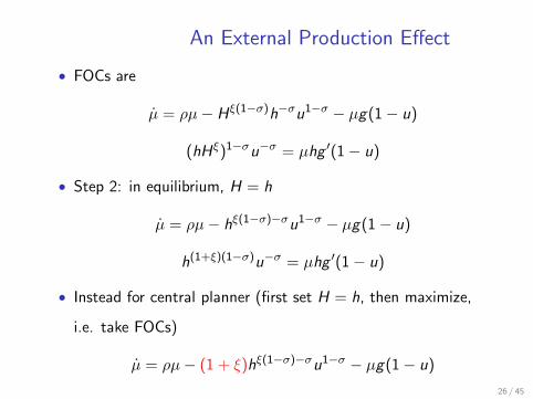
An External Production Effect

• FOCs are

µ = ρµ− Hξ(1−σ)h−σu1−σ− µg(1− u)

(hHξ)1−σu−σ = µhg ′(1− u)

• Step 2: in equilibrium, H = h

µ = ρµ− hξ(1−σ)−σu1−σ− µg(1 − u)

h(1+ξ)(1−σ)u−σ = µhg ′(1− u)

• Instead for central planner (first set H = h, then maximize,

i.e. take FOCs)

µ = ρµ− (1 + ξ)hξ(1−σ)−σu1−σ − µg(1− u)

26 / 45

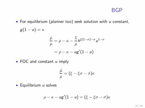
BGP

• For equilibrium (planner too) seek solution with u constant,

g(1− u) = κ

µ

µ= ρ− κ−

1

µhξ(1−σ)−σu1−σ

= ρ− κ− ug ′(1− u)

• FOC and constant u imply

µ

µ= (ξ − ξσ − σ)κ

• Equilibrium u solves

ρ− κ− ug ′(1− u) = (ξ − ξσ − σ)κ

27 / 45

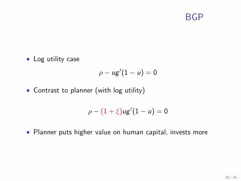
BGP

• Log utility case

ρ− ug ′(1− u) = 0

• Contrast to planner (with log utility)

ρ− (1 + ξ)ug ′(1− u) = 0

• Planner puts higher value on human capital, invests more

28 / 45

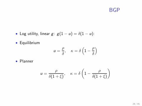
BGP

• Log utility, linear g : g(1− u) = δ(1 − u):

• Equilibrium

u =ρ

δ, κ = δ

(

1−ρ

δ

)

• Planner

u =ρ

δ(1 + ξ), κ = δ

(

1−ρ

δ(1 + ξ)

)

29 / 45

Cross-country income differences?

• Differences in initial, individual h persist forever

• Virtue? Defect? Depends on view on convergence/divergence.

• Migration incentives? Whatever is my h, I am more

productive in economy where H is highest.

30 / 45

(4) An External Learning Effect

• no external effect in production

c = hu

• Instead, external effect appears in the law of motion for h

h = h1−θHθg(1 − u)

• Can work this out as before, results similar.

31 / 45

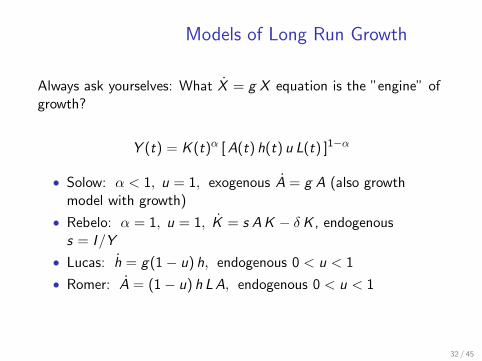
Models of Long Run Growth

Always ask yourselves: What X = g X equation is the ”engine” ofgrowth?

Y (t) = K (t)α [A(t) h(t) u L(t) ]1−α

• Solow: α < 1, u = 1, exogenous A = g A (also growthmodel with growth)

• Rebelo: α = 1, u = 1, K = s AK − δK , endogenouss = I/Y

• Lucas: h = g(1− u) h, endogenous 0 < u < 1

• Romer: A = (1− u) h LA, endogenous 0 < u < 1

32 / 45

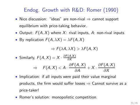
Endog. Growth with R&D: Romer (1990)

• Nice discussion: “ideas” are non-rival ⇒ cannot support

equilibrium with price-taking behavior.

• Output: F (A,X ) where X : rival inputs, A: non-rival inputs

• By replication F (A, λX ) = λF (A,X )

⇒ F (λA, λX ) > λF (A,X )

• Similarly, F (A,X ) = X ·∂F (A,X )

∂X

⇒ F (A,X ) < A ·∂F (A,X )

∂A+ X ·

∂F (A,X )

∂X

• Implication: if all inputs were paid their value marginal

products, the firm would suffer losses ⇒ Cannot survive as a

price-taker!

• Romer’s solution: monopolistic competition.33 / 45

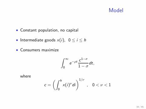
Model

• Constant population, no capital

• Intermediate goods x(i), 0 ≤ i ≤ h

• Consumers maximize

∫ ∞

0e−ρt c

1−σ

1− σdt,

where

c =

(∫ h

0x(i)νdi

)1/ν

, 0 < ν < 1

34 / 45

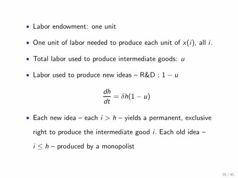
• Labor endowment: one unit

• One unit of labor needed to produce each unit of x(i), all i .

• Total labor used to produce intermediate goods: u

• Labor used to produce new ideas – R&D : 1− u

dh

dt= δh(1− u)

• Each new idea – each i > h – yields a permanent, exclusive

right to produce the intermediate good i . Each old idea –

i ≤ h – produced by a monopolist

35 / 45

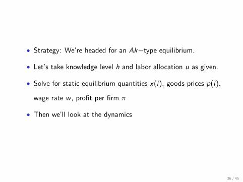
• Strategy: We’re headed for an Ak−type equilibrium.

• Let’s take knowledge level h and labor allocation u as given.

• Solve for static equilibrium quantities x(i), goods prices p(i),

wage rate w , profit per firm π

• Then we’ll look at the dynamics

36 / 45

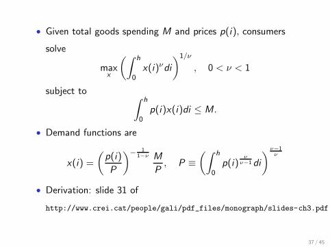
• Given total goods spending M and prices p(i), consumers

solve

maxx

(∫ h

0x(i)νdi

)1/ν

, 0 < ν < 1

subject to∫ h

0p(i)x(i)di ≤ M.

• Demand functions are

x(i) =

(

p(i)

P

)− 11−ν M

P, P ≡

(∫ h

0p(i)

ν

ν−1 di

)

ν−1ν

• Derivation: slide 31 of

http://www.crei.cat/people/gali/pdf_files/monograph/slides-ch3.pdf

37 / 45

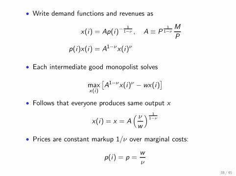
• Write demand functions and revenues as

x(i) = Ap(i)−1

1−ν , A ≡ P1

1−ν

M

P

p(i)x(i) = A1−νx(i)ν

• Each intermediate good monopolist solves

maxx(i)

[

A1−νx(i)ν − wx(i)]

• Follows that everyone produces same output x

x(i) = x = A( ν

w

)1

1−ν

• Prices are constant markup 1/ν over marginal costs:

p(i) = p =w

ν

38 / 45

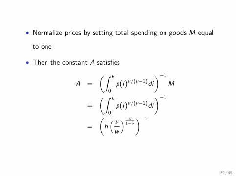
• Normalize prices by setting total spending on goods M equal

to one

• Then the constant A satisfies

A =

(∫ h

0p(i)ν/(ν−1)di

)−1

M

=

(∫ h

0p(i)ν/(ν−1)di

)−1

=

(

h( ν

w

)ν

1−ν

)−1

39 / 45

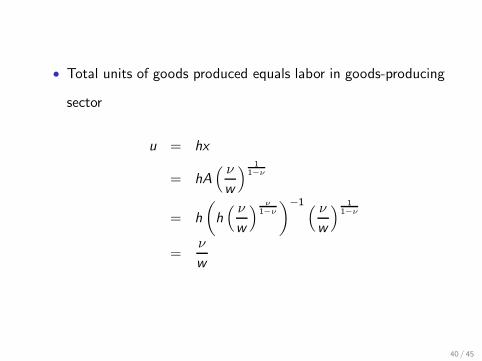
• Total units of goods produced equals labor in goods-producing

sector

u = hx

= hA( ν

w

)1

1−ν

= h

(

h( ν

w

)ν

1−ν

)−1( ν

w

)1

1−ν

=ν

w

40 / 45

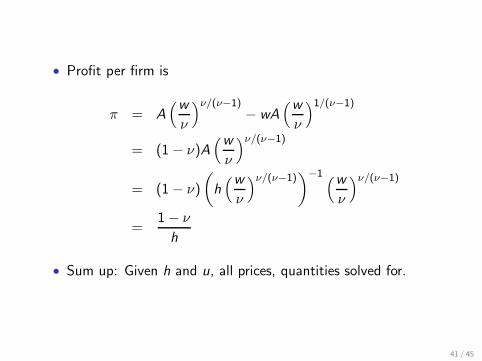
• Profit per firm is

π = A(w

ν

)ν/(ν−1)− wA

(w

ν

)1/(ν−1)

= (1− ν)A(w

ν

)ν/(ν−1)

= (1− ν)

(

h(w

ν

)ν/(ν−1))−1

(w

ν

)ν/(ν−1)

=1− ν

h

• Sum up: Given h and u, all prices, quantities solved for.

41 / 45

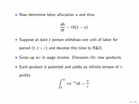
• Now determine labor allocation u and thus

dh

dt= δh(1− u)

• Suppose at date t person withdraw one unit of labor for

period (t, t + ε) and devotes this time to R&D.

• Gives up wε in wage income. Discovers δhε new products.

• Each product is patented and yields an infinite stream of π

profits∫ ∞

0πe−rtdt =

π

r

42 / 45

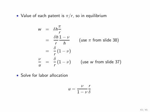
• Value of each patent is π/r , so in equilibrium

w = δhπ

r

=δh

r

1− ν

h(use π from slide 38)

=δ

r(1− ν)

ν

u=

δ

r(1− ν) (use w from slide 37)

• Solve for labor allocation

u =ν

1− ν

r

δ

43 / 45

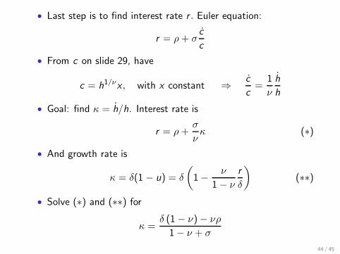
• Last step is to find interest rate r . Euler equation:

r = ρ+ σc

c

• From c on slide 29, have

c = h1/νx , with x constant ⇒c

c=

1

ν

h

h

• Goal: find κ = h/h. Interest rate is

r = ρ+σ

νκ (∗)

• And growth rate is

κ = δ(1 − u) = δ

(

1−ν

1− ν

r

δ

)

(∗∗)

• Solve (∗) and (∗∗) for

κ =δ (1− ν)− νρ

1− ν + σ

44 / 45

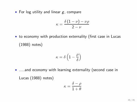
• For log utility and linear g , compare

κ =δ (1− ν)− νρ

2− ν

• to economy with production externality (first case in Lucas

(1988) notes)

κ = δ(

1−ρ

δ

)

• .....and economy with learning externality (second case in

Lucas (1988) notes)

κ =δ − ρ

1 + θ

45 / 45