Lecture 10:

Polynomial Time

Algorithms for Max

Flows

(Reading: AM&O Ch. 7)

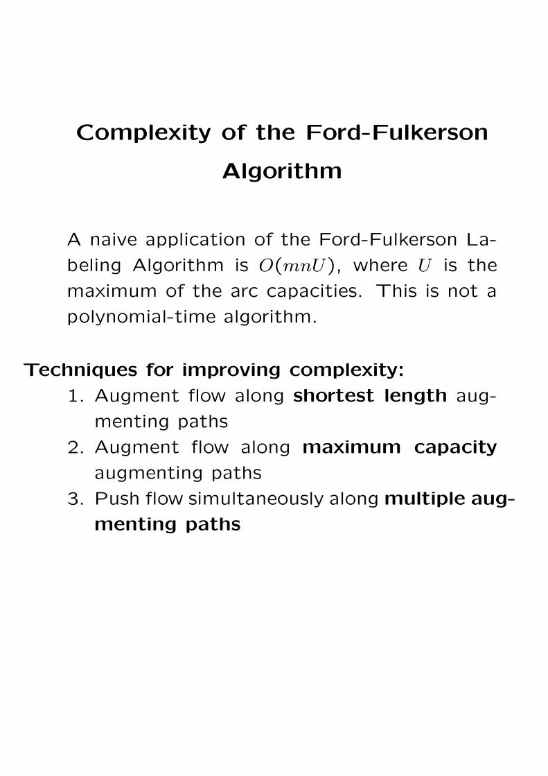
Complexity of the Ford-Fulkerson

Algorithm

A naive application of the Ford-Fulkerson La-

beling Algorithm is O(mnU), where U is the

maximum of the arc capacities. This is not a

polynomial-time algorithm.

Techniques for improving complexity:

1. Augment flow along shortest length aug-

menting paths

2. Augment flow along maximum capacity

augmenting paths

3. Push flow simultaneously along multiple aug-

menting paths

Shortest Length Augmenting

Paths

Fact: If flow is augmented along shortest aug-

menting paths, then max flow is reached after

at most mn/2 flow augmentations.

To prove this, we will give a labeling scheme which

successively finds shortest augmenting paths,

until no more augmenting paths can be found.

At any stage of the F-F Algorithm, let G(x)

be the current residual graph. We maintain a

set d(i) of labels that will be used to find the

length of the shortest (i, t)-path in G(x). The

labels d(i) will always satisfy

d(t) = 0

d(i) ≤ d(j) + 1, (i, j) ∈ G(x)(∗)

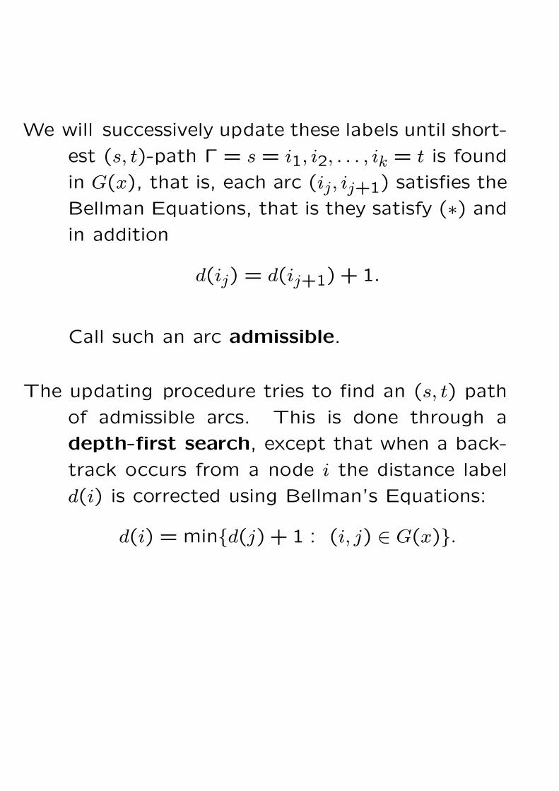
We will successively update these labels until short-

est (s, t)-path Γ = s = i1, i2, . . . , ik = t is found

in G(x), that is, each arc (ij, ij+1) satisfies the

Bellman Equations, that is they satisfy (∗) and

in addition

d(ij) = d(ij+1) + 1.

Call such an arc admissible.

The updating procedure tries to find an (s, t) path

of admissible arcs. This is done through a

depth-first search, except that when a back-

track occurs from a node i the distance label

d(i) is corrected using Bellman’s Equations:

d(i) = min{d(j) + 1 : (i, j) ∈ G(x)}.

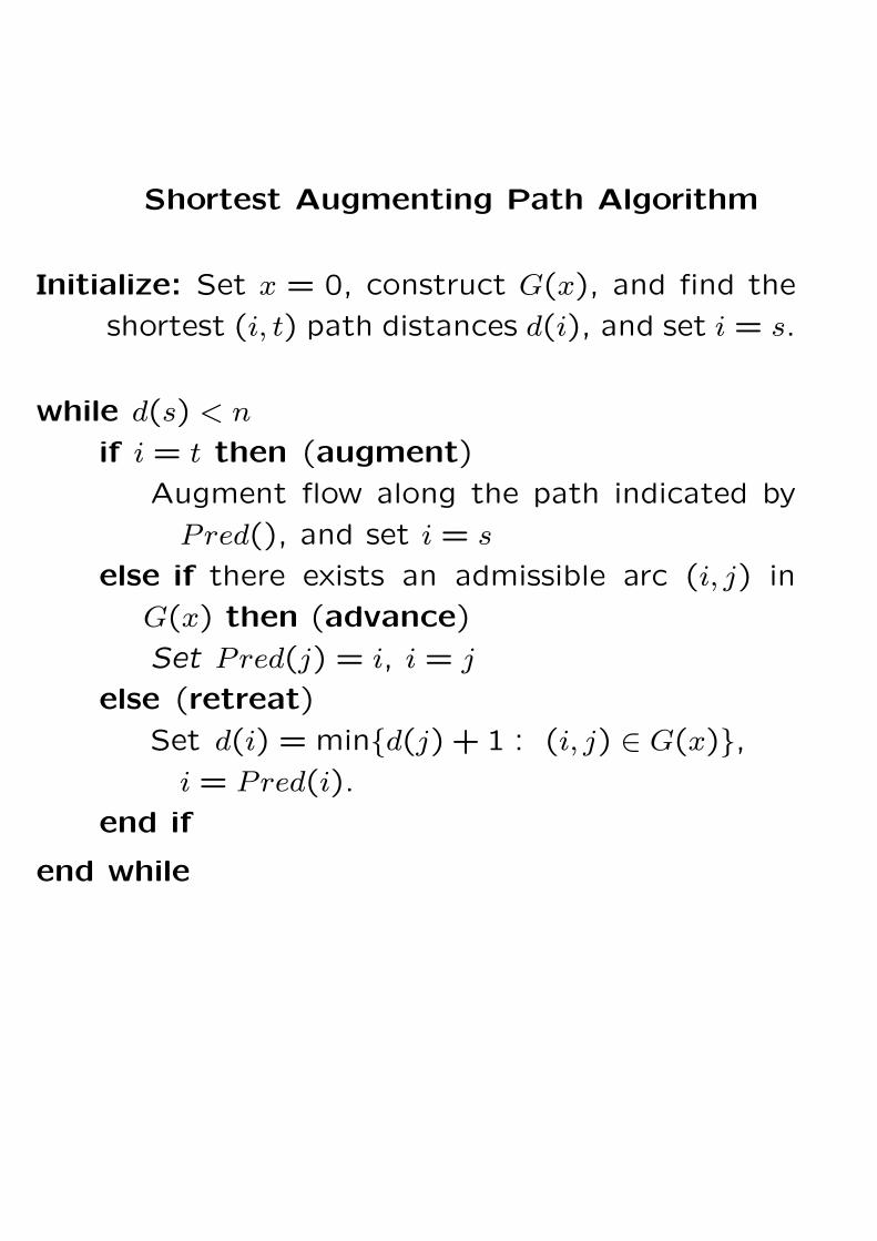
Shortest Augmenting Path Algorithm

Initialize: Set x = 0, construct G(x), and find the

shortest (i, t) path distances d(i), and set i = s.

while d(s) < n

if i = t then (augment)

Augment flow along the path indicated by

Pred(), and set i = s

else if there exists an admissible arc (i, j) in

G(x) then (advance)

Set Pred(j) = i, i = j

else (retreat)

Set d(i) = min{d(j) + 1 : (i, j) ∈ G(x)},i = Pred(i).

end if

end while

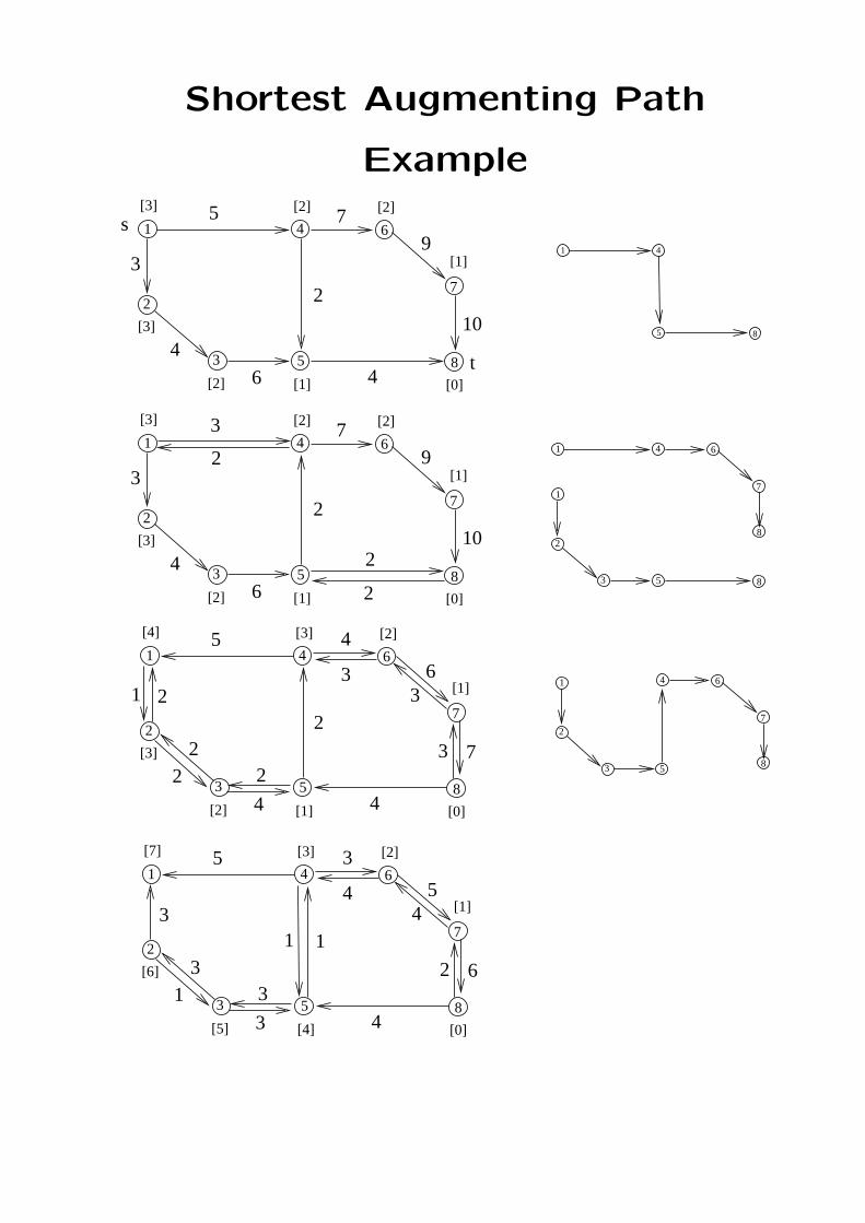
Shortest Augmenting Path

Example

3

1

2

5

4 6

7

9

8

2

[3]

4

1 4 6

7

3

1

2

5 8

8

3

1

2

5

4 6

7

8

1

5

4

8

[2]7

10

[2][3]

[0][2] [1]

3

1

2

5

4 6

7

9[1]

8

2

[3]

6

4

3

3

2

2

2

[2]

t

7

10

4

[2][3]

[0][2] [1]

[1]

5

6

3

[3]

4

[2][7]

[0][5] [4]

3

1

2

5

4 6

7

[1]

8

[6]

5

3

1

3

33

4

2

3

4

1

5

6

1

s

1

[3]

4

[2][4]

[0][2] [1]

3

1

2

5

4 6

7

[1]

8

[3]

5

4

2

2

22

3

3

4

3

2

6

7

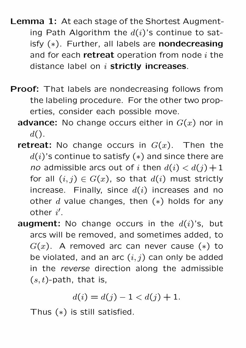
Lemma 1: At each stage of the Shortest Augment-

ing Path Algorithm the d(i)’s continue to sat-

isfy (∗). Further, all labels are nondecreasing

and for each retreat operation from node i the

distance label on i strictly increases.

Proof: That labels are nondecreasing follows from

the labeling procedure. For the other two prop-

erties, consider each possible move.

advance: No change occurs either in G(x) nor in

d().

retreat: No change occurs in G(x). Then the

d(i)’s continue to satisfy (∗) and since there are

no admissible arcs out of i then d(i) < d(j)+1

for all (i, j) ∈ G(x), so that d(i) must strictly

increase. Finally, since d(i) increases and no

other d value changes, then (∗) holds for any

other i′.augment: No change occurs in the d(i)’s, but

arcs will be removed, and sometimes added, to

G(x). A removed arc can never cause (∗) to

be violated, and an arc (i, j) can only be added

in the reverse direction along the admissible

(s, t)-path, that is,

d(i) = d(j)− 1 < d(j) + 1.

Thus (∗) is still satisfied.

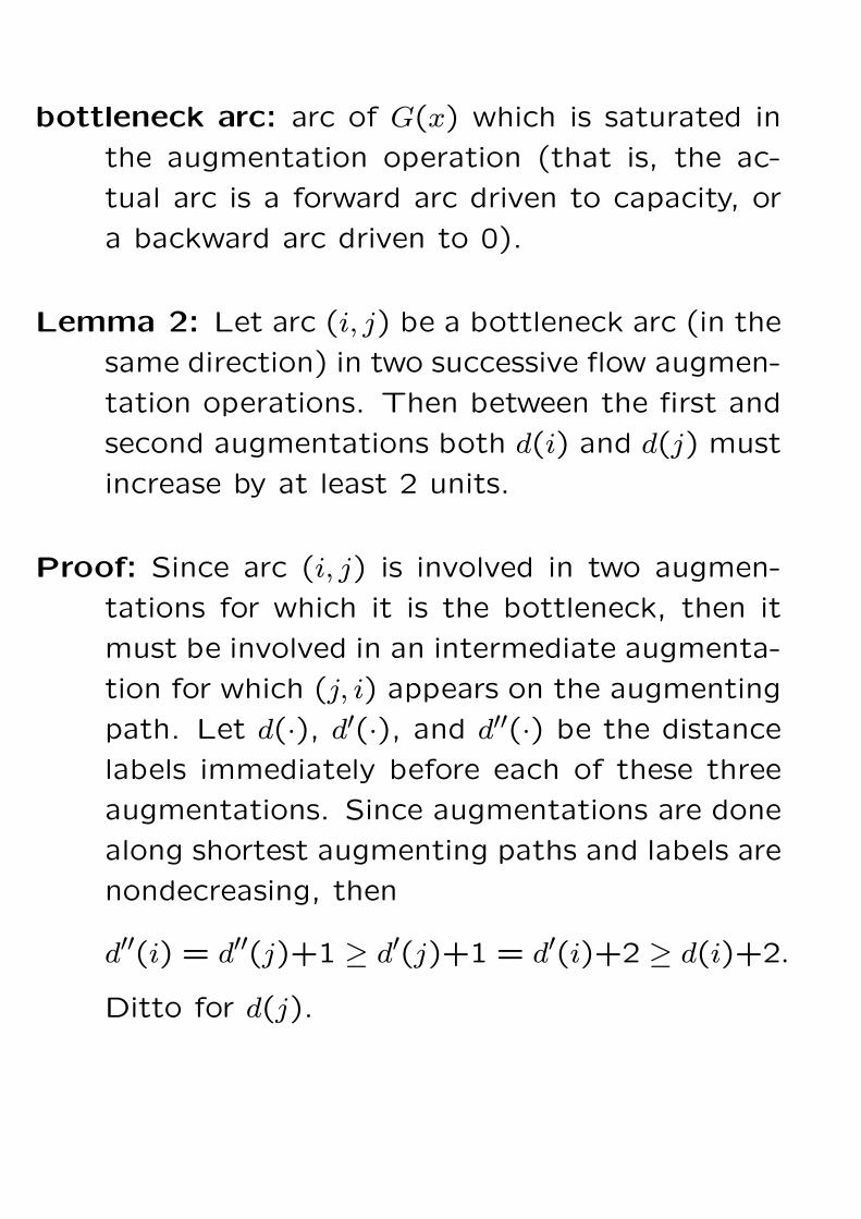
bottleneck arc: arc of G(x) which is saturated in

the augmentation operation (that is, the ac-

tual arc is a forward arc driven to capacity, or

a backward arc driven to 0).

Lemma 2: Let arc (i, j) be a bottleneck arc (in the

same direction) in two successive flow augmen-

tation operations. Then between the first and

second augmentations both d(i) and d(j) must

increase by at least 2 units.

Proof: Since arc (i, j) is involved in two augmen-

tations for which it is the bottleneck, then it

must be involved in an intermediate augmenta-

tion for which (j, i) appears on the augmenting

path. Let d(·), d′(·), and d′′(·) be the distance

labels immediately before each of these three

augmentations. Since augmentations are done

along shortest augmenting paths and labels are

nondecreasing, then

d′′(i) = d′′(j)+1 ≥ d′(j)+1 = d′(i)+2 ≥ d(i)+2.

Ditto for d(j).

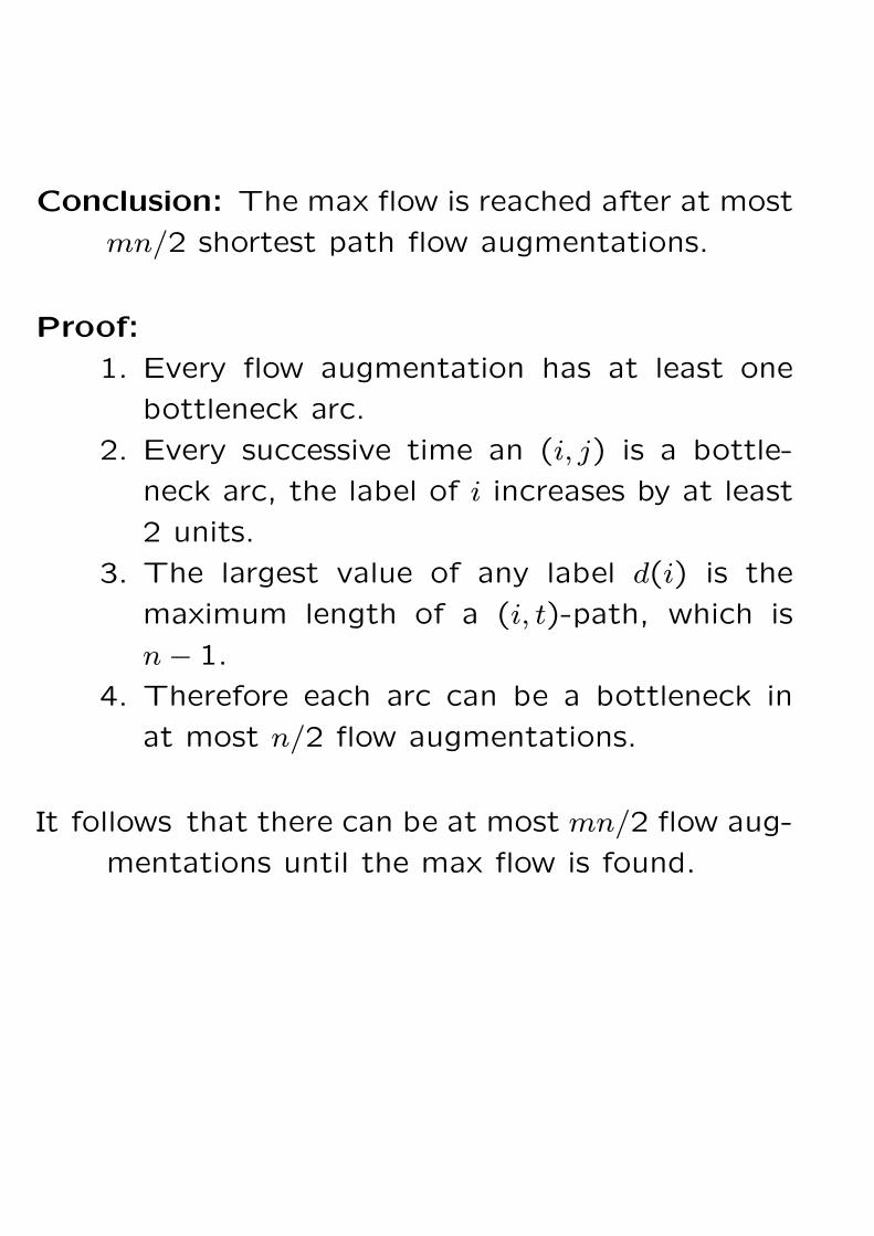
Conclusion: The max flow is reached after at most

mn/2 shortest path flow augmentations.

Proof:

1. Every flow augmentation has at least one

bottleneck arc.

2. Every successive time an (i, j) is a bottle-

neck arc, the label of i increases by at least

2 units.

3. The largest value of any label d(i) is the

maximum length of a (i, t)-path, which is

n− 1.

4. Therefore each arc can be a bottleneck in

at most n/2 flow augmentations.

It follows that there can be at most mn/2 flow aug-

mentations until the max flow is found.

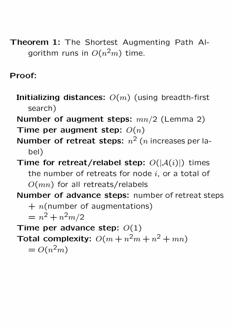
Theorem 1: The Shortest Augmenting Path Al-

gorithm runs in O(n2m) time.

Proof:

Initializing distances: O(m) (using breadth-first

search)

Number of augment steps: mn/2 (Lemma 2)

Time per augment step: O(n)

Number of retreat steps: n2 (n increases per la-

bel)

Time for retreat/relabel step: O(|A(i)|) times

the number of retreats for node i, or a total of

O(mn) for all retreats/relabels

Number of advance steps: number of retreat steps

+ n(number of augmentations)

= n2 + n2m/2

Time per advance step: O(1)

Total complexity: O(m+ n2m+ n2 +mn)

= O(n2m)

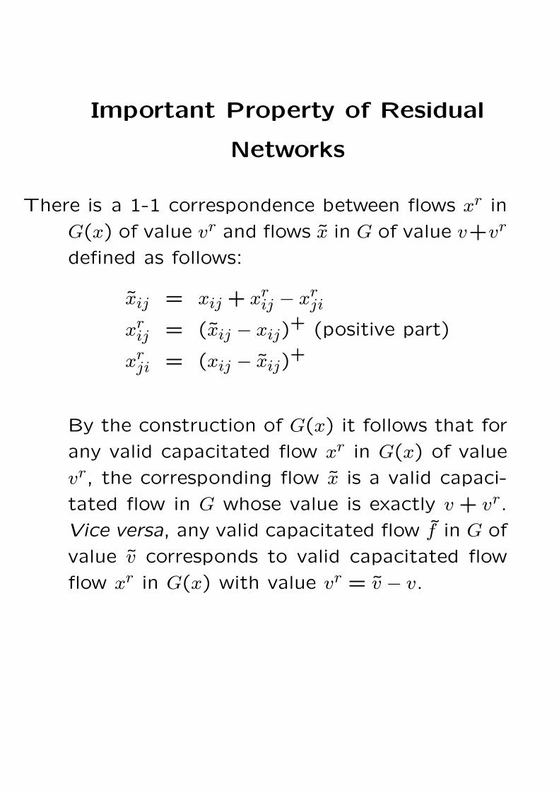
Important Property of Residual

Networks

There is a 1-1 correspondence between flows xr in

G(x) of value vr and flows x in G of value v+vr

defined as follows:

xij = xij + xrij − xrji

xrij = (xij − xij)+ (positive part)

xrji = (xij − xij)+

By the construction of G(x) it follows that for

any valid capacitated flow xr in G(x) of value

vr, the corresponding flow x is a valid capaci-

tated flow in G whose value is exactly v + vr.

Vice versa, any valid capacitated flow f in G of

value v corresponds to valid capacitated flow

flow xr in G(x) with value vr = v − v.

5,6

64

Residual network

71

5

11

8

2

6,10

~

8,10 8,8

0,1

6,6

1,1

1,1

1,1

Flow

New flowCurrent flow

6,10

8,10

64

7

5

8

2

1,1

7,8

uij

r

x

ijxijr

,ij ijx

4

4

3

2

1

1

2

3

41

3

2

4

3

2

1

In particular, if xr = x∗ is the max flow in G(x) of

value v∗, then the corresponding flow x in G

must be a max flow as well, with value v∗ + v.

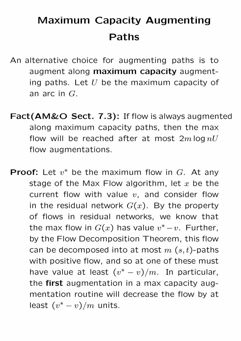
Maximum Capacity Augmenting

Paths

An alternative choice for augmenting paths is to

augment along maximum capacity augment-

ing paths. Let U be the maximum capacity of

an arc in G.

Fact(AM&O Sect. 7.3): If flow is always augmented

along maximum capacity paths, then the max

flow will be reached after at most 2m lognU

flow augmentations.

Proof: Let v∗ be the maximum flow in G. At any

stage of the Max Flow algorithm, let x be the

current flow with value v, and consider flow

in the residual network G(x). By the property

of flows in residual networks, we know that

the max flow in G(x) has value v∗−v. Further,

by the Flow Decomposition Theorem, this flow

can be decomposed into at most m (s, t)-paths

with positive flow, and so at one of these must

have value at least (v∗ − v)/m. In particular,

the first augmentation in a max capacity aug-

mentation routine will decrease the flow by at

least (v∗ − v)/m units.

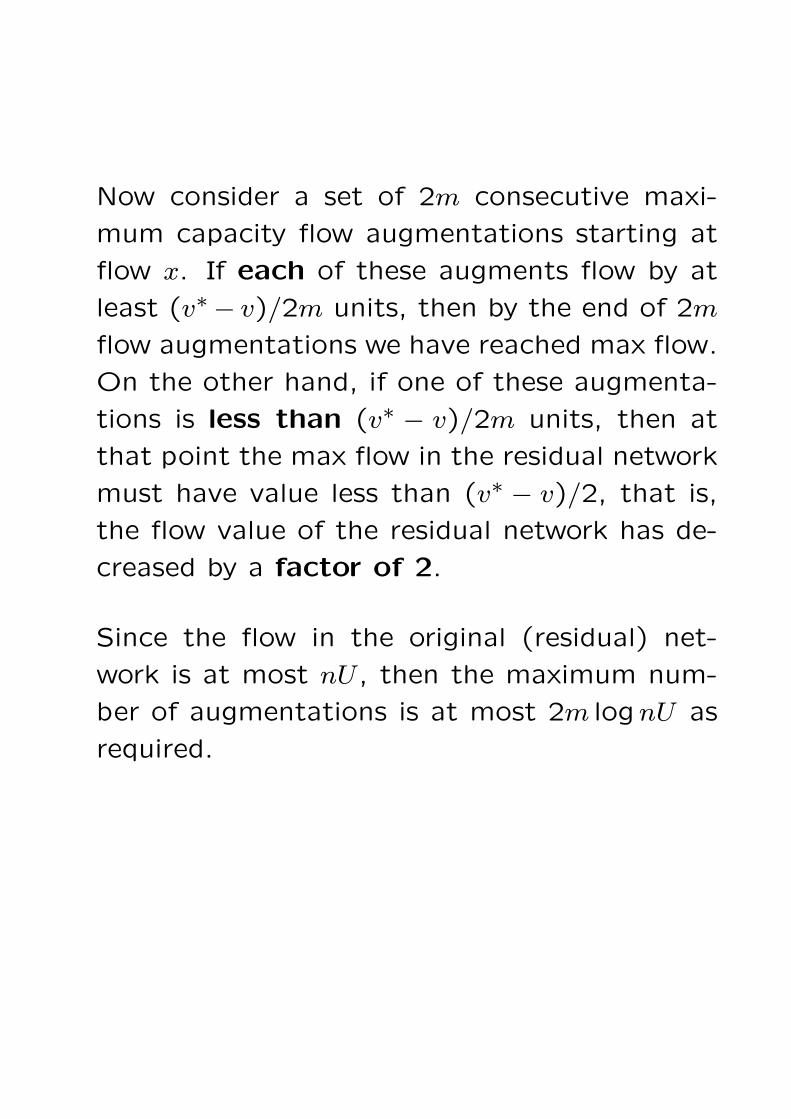
Now consider a set of 2m consecutive maxi-

mum capacity flow augmentations starting at

flow x. If each of these augments flow by at

least (v∗− v)/2m units, then by the end of 2m

flow augmentations we have reached max flow.

On the other hand, if one of these augmenta-

tions is less than (v∗ − v)/2m units, then at

that point the max flow in the residual network

must have value less than (v∗ − v)/2, that is,

the flow value of the residual network has de-

creased by a factor of 2.

Since the flow in the original (residual) net-

work is at most nU , then the maximum num-

ber of augmentations is at most 2m lognU as

required.

Conclusion: The implementation of the Max Flow

Algorithm using maximum capacity augment-

ing paths has complexity O(m(m+n logn) lognU),

(using Fibonacci heaps).

Bottleneck: Finding max capacity augmenting paths

is expensive.

Solution: Find “large capacity” augmenting paths

instead. More specifically,

ith scaling phase: Find all augmenting paths

of capacity at least ∆ = U/2i.

This is done by considering the ∆-residual

network G(x,∆) of edges of G(x) having ca-

pacity at least ∆. G(x,∆) can be constructed

and updated in O(m) time, and the appropri-

ate path is found by applying FINDPATH to

G(f,∆).

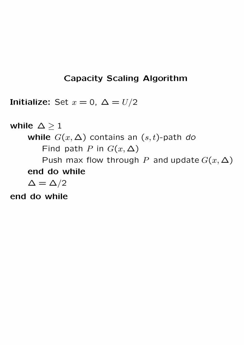
Capacity Scaling Algorithm

Initialize: Set x = 0, ∆ = U/2

while ∆ ≥ 1

while G(x,∆) contains an (s, t)-path do

Find path P in G(x,∆)

Push max flow through P and update G(x,∆)

end do while

∆ = ∆/2

end do while

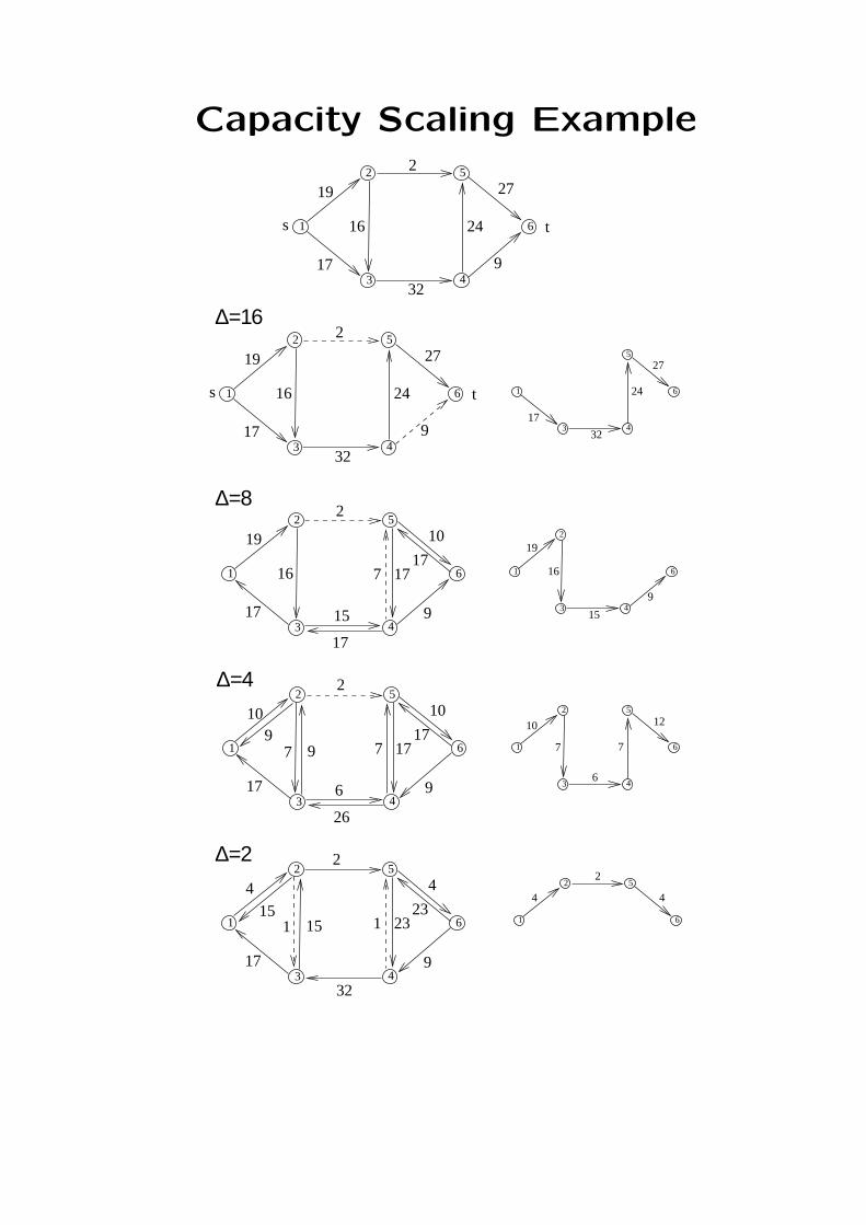
Capacity Scaling Example

1

2

3

6

4

52

32

24

27

9

19

17

16 ts

3 432

917

1

2

6

5

24

2719

16

1

2

6

52

4 4

3 4

1

2

6

5

10

7

6

7

12

3 415

9

1

2

6

19

16

3 432

17

1 6

5

24

27

ts

2∆=16

∆=8

3 4

1

2

6

5

4

1

4

9

2323

∆=2

1 15

32

3 417

1

2

6

5

10

7

6

10

9

26

1717

∆=4

97 9

17

15

3 417

1

2

6

5

19

16 7

15

10

9

17

1717

2

2

2

Theorem 2: The capacity scaling algorithm solves

the maximum flow problem in O(m2 logU) time.

Proof: We show that the algorithm performs at

most 2m augmentations during each scaling

phase. At the end of the ith scaling phase

with value ∆ there are no more (s, t)-paths in

G(x,∆). By the Duality Theorem for (s, t)-

paths, this means that there must be an (s, t)-

cut (X, X) having no arcs of G(x,∆), i.e., all

arcs of G(x) in (X, X) have capacity less than

∆. This means that the max flow in G(x)

can be at most the capacity of (X, X) in G(x),

which is in turn less than m∆. Now consider

the (i+1)st scaling phase. Since the max flow

in G(x) is at at most m∆, and the capacity

of every augmenting path is at least ∆/2 in

this phase, then there can be at most 2m flow

augmentations occurring in this phase.

Since there are at most logU scaling phases

then there are at most 2m logU flow augmen-

tations. Finding the paths in G(x,∆) requires

O(m) time, for a total of O(m2 logU) for the

algorithm.

Improving Capacity Scaling to O(mn logU): Use

the Shortest Augmenting Path Algorithm

to send flow along shortest augmenting paths

in G(x,∆). Since the number of augmenta-

tions in each scaling phase is at most 2m, then

the number of augment and advance steps per

scaling phase is now 2m and 2mn, respectively,

for a total of O(m + mn + n2) = O(mn) per

scaling phase, or O(mn logU) overall.

Other Improvements

Augmenting along Multiple Paths:

Idea: Push as much flow as you can through all

augmenting paths simultaneously, by push-

ing flow along individual arcs subject to capac-

ity and “throughput constraints”.

Pre-flow Push: Instead of reconstructing the shortest-

path network each time, modify the Shortest

Path Algorithm to allow you to augment flow

through all shortest paths while you update

labels. This involves a “two-wave” process,

pushing flow toward t — possibly leaving ex-

cess flow at nodes — and then going back

toward s correcting any excess flow at each

node.

Complexity: Depends upon the search order.

“Generic” Preflow-Push: O(n2m)

Dinic’s Algorithm (FIFO Preflow Push im-

plementation): Construct the subnetwork Gs

of G(x) consisting of all shortest length (aug-

menting) paths. Pre-flow push can be imple-

mented to find the max flow in Gs in O(n2)

time.) Repeat this for successively longer paths

(using a variant of Lemma 2), until the longest

— i.e. (n − 1)-arc — paths have been satu-

rated. Total complexity: O(n3) (See AM&O,

Sections 7.5&7.7)

“Highest Label” Preflow-Push: O(n2√m))

“Excess Scaling” Preflow-Push:

O(nm+ n2 logU)

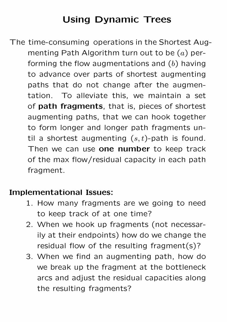
Using Dynamic Trees

The time-consuming operations in the Shortest Aug-

menting Path Algorithm turn out to be (a) per-

forming the flow augmentations and (b) having

to advance over parts of shortest augmenting

paths that do not change after the augmen-

tation. To alleviate this, we maintain a set

of path fragments, that is, pieces of shortest

augmenting paths, that we can hook together

to form longer and longer path fragments un-

til a shortest augmenting (s, t)-path is found.

Then we can use one number to keep track

of the max flow/residual capacity in each path

fragment.

Implementational Issues:

1. How many fragments are we going to need

to keep track of at one time?

2. When we hook up fragments (not necessar-

ily at their endpoints) how do we change the

residual flow of the resulting fragment(s)?

3. When we find an augmenting path, how do

we break up the fragment at the bottleneck

arcs and adjust the residual capacities along

the resulting fragments?

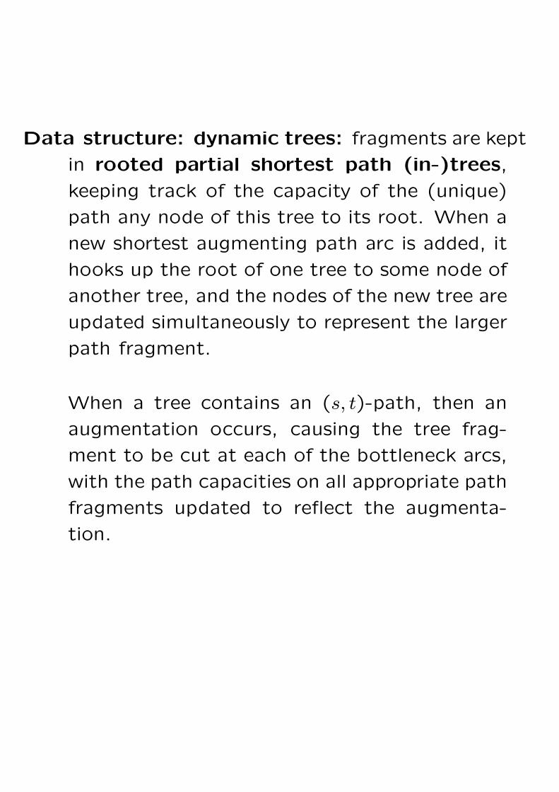
Data structure: dynamic trees: fragments are kept

in rooted partial shortest path (in-)trees,

keeping track of the capacity of the (unique)

path any node of this tree to its root. When a

new shortest augmenting path arc is added, it

hooks up the root of one tree to some node of

another tree, and the nodes of the new tree are

updated simultaneously to represent the larger

path fragment.

When a tree contains an (s, t)-path, then an

augmentation occurs, causing the tree frag-

ment to be cut at each of the bottleneck arcs,

with the path capacities on all appropriate path

fragments updated to reflect the augmenta-

tion.

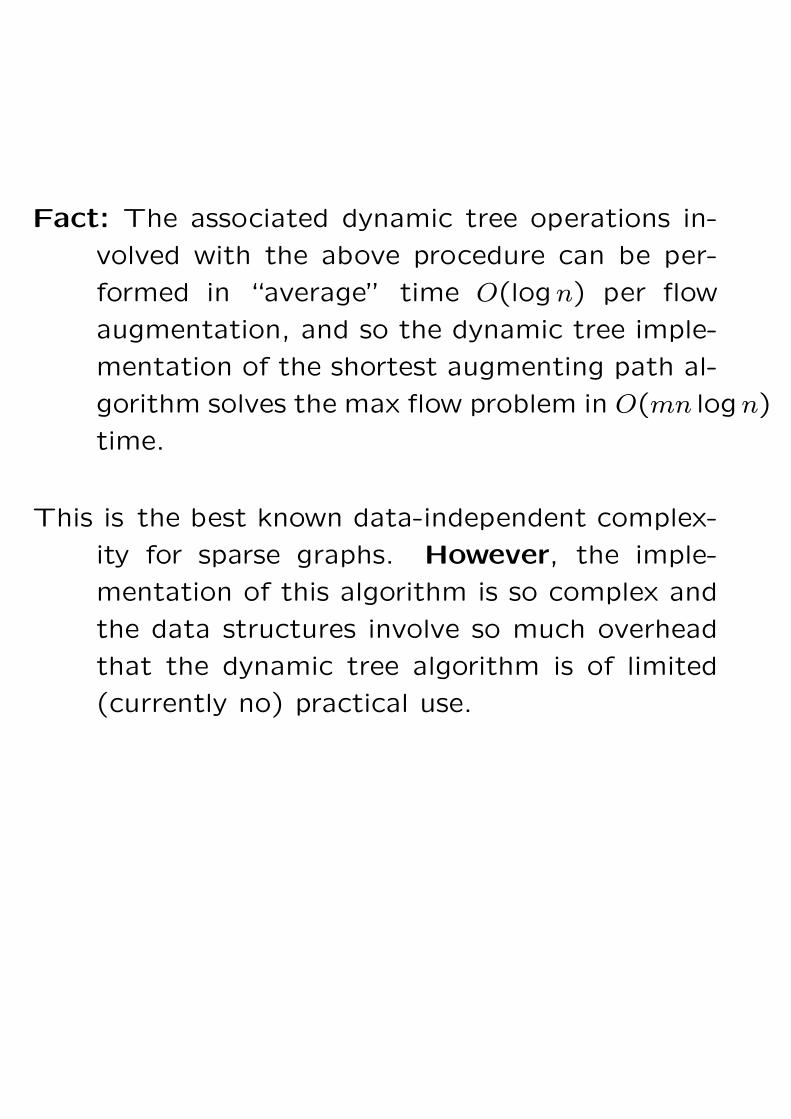
Fact: The associated dynamic tree operations in-

volved with the above procedure can be per-

formed in “average” time O(logn) per flow

augmentation, and so the dynamic tree imple-

mentation of the shortest augmenting path al-

gorithm solves the max flow problem in O(mn logn)

time.

This is the best known data-independent complex-

ity for sparse graphs. However, the imple-

mentation of this algorithm is so complex and

the data structures involve so much overhead

that the dynamic tree algorithm is of limited

(currently no) practical use.

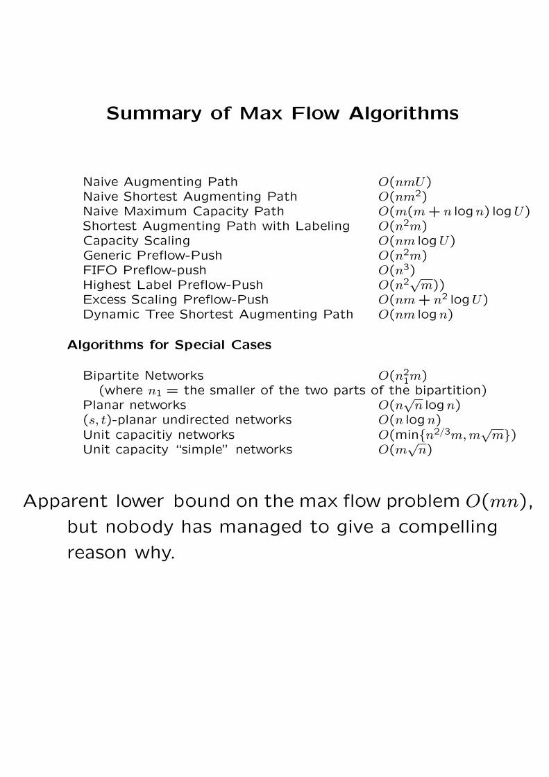
Summary of Max Flow Algorithms

Naive Augmenting Path O(nmU)Naive Shortest Augmenting Path O(nm2)Naive Maximum Capacity Path O(m(m+ n logn) logU)Shortest Augmenting Path with Labeling O(n2m)Capacity Scaling O(nm logU)Generic Preflow-Push O(n2m)FIFO Preflow-push O(n3)Highest Label Preflow-Push O(n2√m))Excess Scaling Preflow-Push O(nm+ n2 logU)Dynamic Tree Shortest Augmenting Path O(nm logn)

Algorithms for Special Cases

Bipartite Networks O(n21m)

(where n1 = the smaller of the two parts of the bipartition)Planar networks O(n

√n logn)

(s, t)-planar undirected networks O(n logn)Unit capacitiy networks O(min{n2/3m,m

√m})

Unit capacity “simple” networks O(m√n)

Apparent lower bound on the max flow problem O(mn),

but nobody has managed to give a compelling

reason why.