MLISP: Machine Learning in Signal Processing Lecture 11 Prof. V. I. Morgenshtern Scribe: M. Elminshawi Illustrations: The elements of statistical learning, Hastie, Tibshirani, Friedman Agenda 1. Wavelets with good frequency localization 2. Wavelet transform of NMR signal 3. Denoising via wavelet shrinkage 1 Wavelets with good frequency localization Haar wavelets are simple to understand, but they are not smooth enough for most purposes. The Daubechies symmlet-8 wavelets, constructed in a similar way, have the same orthonormal properties as Haar wavelets, but are smoother. Here is the comparison of father functions for the two systems: and here are the shifts: 1
Transcript
MLISP: Machine Learning in Signal Processing
Lecture 11
Prof. V. I. Morgenshtern
Scribe: M. Elminshawi
Illustrations: The elements of statistical learning, Hastie, Tibshirani, Friedman
Agenda
1. Wavelets with good frequency localization
2. Wavelet transform of NMR signal
3. Denoising via wavelet shrinkage
1 Wavelets with good frequency localization
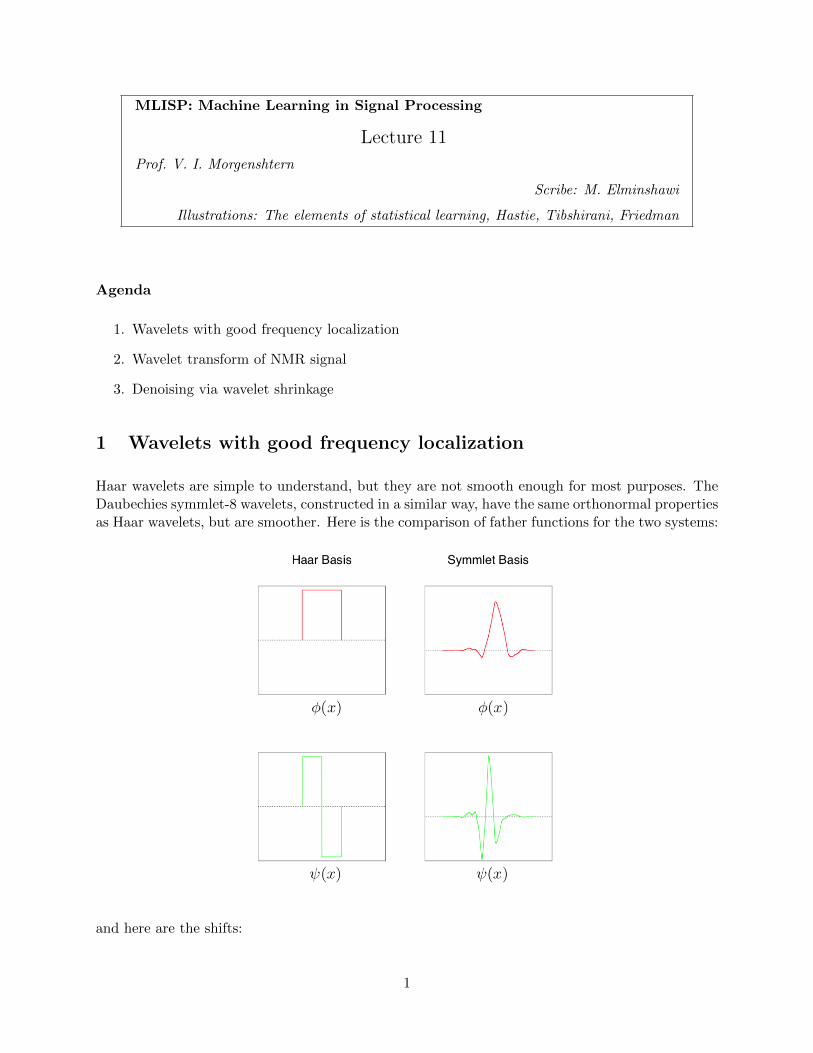
Haar wavelets are simple to understand, but they are not smooth enough for most purposes. TheDaubechies symmlet-8 wavelets, constructed in a similar way, have the same orthonormal propertiesas Haar wavelets, but are smoother. Here is the comparison of father functions for the two systems:
and here are the shifts:
1
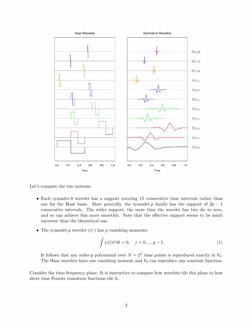
Let’s compare the two systems:
• Each symmlet-8 wavelet has a support covering 15 consecutive time intervals rather thanone for the Haar basis. More generally, the symmlet-p family has the support of 2p − 1consecutive intervals. The wider support, the more time the wavelet has two die to zero,and so can achieve this more smoothly. Note that the effective support seems to be muchnarrower than the theoretical one.
• The symmlet-p wavelet ψ(·) has p vanishing moments:∫ψ(t)tjdt = 0, j = 0, ..., p− 1. (1)
It follows that any order-p polynomial over N = 2J time points is reproduced exactly in V0.The Haar wavelets have one vanishing moment and V0 can reproduce any constant function.
Consider the time-frequency plane. It is instructive to compare how wavelets tile this plane to howshort time Fourier transform functions tile it:
2
We observe that in the case of wavelets every time we go up the hierarchy stack, the number offunctions doubles, each function becomes more localized (more narrow), and therefore it’s frequencycontent doubles.
2 Wavelet transform of NMR signal
In the following figure we see an NMR (nuclear magnetic resonance) signal, which appears to becomposed of smooth components and isolated spikes, plus some noise:
3
The wavelet transform using Symmlet basis, is shown in the lower left panel:
The wavelet coefficients are arranged in rows, from lowest scale at the bottom to highest scale at thetop. The length of each line segment indicates the size of the coefficients. These rows correspondto the decomposition:
signal span = V4 ⊕W4 ⊕W5 ⊕W6 ⊕W7 ⊕W8 ⊕W9 (2)
that we studied before.
The bottom right panel shows the wavelet coefficients after they have been thresholded via soft-thresholding (will study next). Note that many of the smaller coefficients have been set to zero.The green curve in the top panel shows inverse transform of the thresholded coefficients. This isthe denoised version of the original signal.
3 Denoising via wavelet shrinkage
Let’s now give a mathematically precise method to obtain the wavelet smoothing. Suppose ourNMR signal (rescaled to live on the interval [0, 1]), is sampled at N = 2J lattice points; call thediscrete signal y. Since wavelets form an orthonormal basis, we can stack the wavelet basis functionsinto an orthogonal matrix WT. Each row of WT is one wavelet basis function, sampled at the
Note that the matrix W is a square matrix of size 2J × 2J . Then y∗ = WTy is called the discretewavelet transform of y. Here is a signal y at the top and it’s wavelet transform coefficients arrangedby scale in the remaining rows:
Notice that in this representation, the coefficients do not descent all way to V0 but stop at V4 whichhas 16 basis functions. As we ascend to each new level of detail, the coefficients get smaller, exceptin the locations where spiky behavior is present.
5
We would like to somehow capture the fact that the true signal should have few nonzero coefficientsonly those that correspond to spiky behavior.
One approach to do this is to solve:
minθ
‖y −Wθ‖22︸ ︷︷ ︸least squares regression term
+ 2λ · (# of nonzero elements in θ)︸ ︷︷ ︸regularization term
.
Above, y is the noisy data, W is the transformation matrix from the wavelet domain to the signaldomain, θ is the vector of estimated wavelet coefficients, λ is the parameter that controls thetrade-off between data fidelity and sparsity.
Unfortunately, the above optimization problem is computationally infeasible! It is non-convex andeven non-smooth; we cannot use the gradient descent. Instead we solve this:
minθ
‖y −Wθ‖22 + 2λ ‖θ‖1 . (3)
where the ‖θ‖1 is the term that promotes sparsity as we will shortly see.
In general, the optimization problem of form (3) is convex, and therefore the minimum can easilybe found numerically. The case we are considering now is special, because W is an orthogonalmatrix. In this case, the solution can be found analytically as follows. First note that since W isorthogonal, it does not change the norm of a vector so that:
‖y −Wθ‖22 =∥∥∥WT(y −Wθ)
∥∥∥22
=
∥∥∥∥∥∥WTy −WTW︸ ︷︷ ︸I
θ
∥∥∥∥∥∥2
2
=∥∥∥WTy − θ
∥∥∥22
= ‖y∗ − θ‖22 .
Hence, (3) is equivalent to:min
θ
‖y∗ − θ‖22 + 2λ ‖θ‖1
which can be written as
minθ
N∑i=1
(y∗i − θi)2 + 2λN∑i=1
|θi|.
Therefore, the problem decouples and we just need to solve:
minθi
(y∗i − θi)2 + 2λ|θi|
for each i separately.
Let f(θ) = (y∗− θ)2 + 2λ|θ|. What is the minimum of f(θ)? To find the minimum of this function,take the derive and set it to zero:
f ′(θ) = −2(y∗ − θ) + 2λ sign θ
where we used |θ|′ = sign(θ) as can be seen from the plot:
6
We find, f ′(θ) = 0 iff−y∗ + θ + λ sign θ = 0. (4)
Claim: The solution to (4) isθ∗ = sign(y∗)(|y∗| − λ)+, (5)
where
(u)+ =
{u, u > 0
0, otherwise.
Proof. If θ > 0, then (4) is equivalent to:
− y∗ + θ + λ = 0
⇔ θ = y∗ − λ⇔ θ = (y∗ − λ)+
⇔ θ = sign(y∗)(|y∗| − λ)+
where the last step follows because θ = y∗ − λ > 0⇒ y∗ > λ > 0⇒ sign(y∗) = 1.
If θ < 0, then (4) is equivalent to:
− y∗ + θ − λ = 0
⇔ θ = y∗ + λ
⇔ θ = sign(y∗)(|y∗| − λ)+
where the last step follows because θ = y∗ + λ < 0 ⇒ y∗ < −λ < 0 ⇒ sign(y∗) = −1 and also|y∗| = −y∗.
What is the meaning of the formula (5)?
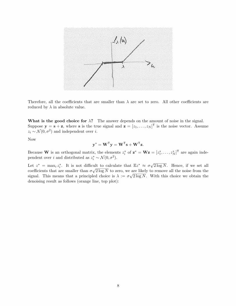
The function fλ(u) = sign(u)(|u| − λ)+ is called the soft-thresholding function. It looks like this:
7
Therefore, all the coefficients that are smaller than λ are set to zero. All other coefficients arereduced by λ in absolute value.
What is the good choice for λ? The answer depends on the amount of noise in the signal.Suppose y = s + z, where s is the true signal and z = [z1, . . . , zN ]T is the noise vector. Assumezi ∼ N (0, σ2) and independent over i.
Nowy∗ = WTy = WTs + WTz.
Because W is an orthogonal matrix, the elements z∗i of z∗ = Wz = [z∗1 , . . . , z∗N ]T are again inde-
pendent over i and distributed as z∗i ∼ N (0, σ2).
Let z∗ = maxi z∗i . It is not difficult to calculate that Ez∗ ≈ σ
√2 logN . Hence, if we set all
coefficients that are smaller than σ√
2 logN to zero, we are likely to remove all the noise from thesignal. This means that a principled choice is λ := σ
√2 logN . With this choice we obtain the
denoising result as follows (orange line, top plot):
8
Let’s compare the spline and the wavelet smoothing for two different signals as in the figure above.In NMR example, splines introduce many unnecessary features. Wavelets fit nicely localized spikes.In the second plot, the true function is smooth and the noise is high. The wavelet fit has leftunnecessary wiggles - a price it pays in variance for additional adaptivity.