Lecture #12 of 26

10/30/2020

1

391

Lecture #12 of 26

392

Time-Dependence in Electrochemistry

Chapters 4 and 5

393

Q: What’s in this set of lectures?A: B&F Chapters 4 & 5 main concepts:

● Section 4.4.2: Fick’s Second Law of Diffusion

● Section 5.1: Overview of step experiments

● Section 5.2: Potential step under diffusion controlled

● Sections 5.3 & 5.9:Ultramicroelectrodes

● Sections 5.7 – 5.8: Chronoamperometry/Chronocoulometry

10/30/2020

2

394

Looking forward… Section 4.4.2 and Chapter 5

● Fick’s Second Law of Diffusion

● Linear Diffusion = time-dependent current (Cottrell Equation)

● Anson Plots for surface adsorbed species

● Radial Diffusion = time-independent current (at steady-state)

● Ultramicroelectrodes (UMEs)

● Scanning Electrochemical Microscopy (SECM)

● Single molecule electrochemistry

395

Fick’s 1st Law of Diffusion:Adolph Eugen Fick

… but taking baby steps toward theCottrell equation… conceptually, one canderive Fick’s law in a manner similar tohow we thought about the diffusioncoefficient… grab your favorite beverageand go on a walk!

We use both of Fick’s laws of diffusion to derive equations for time-dependent (not steady-state) transport-controlled electrochemistry...

B&F, pg. 149

the Cottrell Equation… and here’s the conclusion of that derivation…

396


This is the net flux (correct dimensions)…… with half moving right and half moving left

B&F, pg. 149


10/30/2020

3

397


B&F, pg. 149

… derived!Recall…


398

Fick’s 1st Law of Diffusion:

Fick’s 2nd Law of Diffusion:

Adolph Eugen Fick

… derive this non-steady-stateequation (approximately) in asimilar fashion as Fick’s first law…

B&F, pg. 149


399… the derivation is not so bad…

B&F, pp. 149–150

10/30/2020

4

400

(First Law)

… derived!

B&F, pp. 149–150

… the derivation is not so bad…

401The experiment we will model is a potential step experiment…key points: at E1: no reaction (CO(x, 0) = CO*)

at E2: diffusion-controlled reaction (CO(0, t) = 0)

Eeq

> 200 mV

> 200 mV

How to derive expressions for diffusion-controlled current vs. time: 402

1. Solve Fick’s Second Law to get CO(x, t), and in the process of doing this, you will use boundary conditions that “customize” the solution for the particular experiment of interest:

3. Calculate the time-dependent diffusion-limited current:

i = nFAJO(0, t)

2. Use Fick’s First Law to calculate JO(0, t) from CO(x, t):

… using the… Laplace transform, integration by parts, L’Hôpital’s rule, Schrödingerequation, complementary error function, Leibniz rule, chain rule… Wow! Cool!

10/30/2020

5

403

how about F(t) = 1?

Step 1 is the kicker… we’ll use the Laplace Transform to solve thelinear partial differential equation

The Laplace transform of any function F(t) is:

𝐿 1 = න

0

∞

𝑒−𝑠𝑡 1 𝑑𝑡 = อ𝑒−𝑠𝑡

−𝑠0

∞

= 0 −1

−𝑠=1

𝑠

𝐿 𝑘𝑡 = න

0

∞

𝑒−𝑠𝑡 𝑘𝑡 𝑑𝑡 = 𝑘න

0

∞

𝑡𝑒−𝑠𝑡𝑑𝑡 = อ𝑘𝑒−𝑠𝑡

𝑠2−𝑠𝑡 − 1

0

∞

how about F(t) = kt?

404

how about F(t) = e–at?

how about F(t) = kt? Integrated by parts

Used L’Hôpital’s rule

𝐿 𝑘𝑡 = න

0

∞

𝑒−𝑠𝑡 𝑘𝑡 𝑑𝑡 = 𝑘න

0

∞

𝑡𝑒−𝑠𝑡𝑑𝑡 = อ𝑘𝑒−𝑠𝑡

𝑠2−𝑠𝑡 − 1

0

∞

= 𝑘 0 −1

𝑠2−1 =

𝑘

𝑠2

𝐿 𝑒−𝑎𝑡 = න

0

∞

𝑒−𝑠𝑡𝑒−𝑎𝑡𝑑𝑡 = න

0

∞

𝑒− 𝑠+𝑎 𝑡𝑑𝑡 = อ𝑒− 𝑠+𝑎 𝑡

− 𝑠 + 𝑎0

∞

= 0 −1

− 𝑠 + 𝑎=

1

𝑠 + 𝑎

405

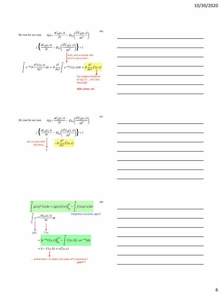
OK, now for our case:

Recall, Second Law:

–F(t) =

10/30/2020

6

406

the Laplace transformof C(x, t)? … Isn’t this cheating?

Well, ahem, no!


well, wait a second, thisterm is not so bad…

–F(t) =

–L{ }= ?

න

0

∞

𝑒−𝑠𝑡𝐷𝜕2𝐶 𝑥, 𝑡

𝜕𝑥2𝑑𝑡 = 𝐷

𝜕2

𝜕𝑥2න

0

∞

𝑒−𝑠𝑡𝐶 𝑥, 𝑡 𝑑𝑡 = 𝐷𝜕2

𝜕𝑥2ҧ𝐶 𝑥, 𝑠

407

?


not so lucky with this term…

–F(t) =

–L{ }= ?

−𝐷𝜕2


408

… and at time = 0, what is the value of C, anywhere?… just C*!

Integration, by parts, again!

g(x) f '(x)

න

0

∞

𝑒−𝑠𝑡𝜕𝐶𝑂 𝑥, 𝑡

𝜕𝑡𝑑𝑡

න

𝑎

𝑏

𝑔 𝑥 𝑓′ 𝑥 𝑑𝑥 = ቚ𝑔 𝑥 𝑓 𝑥𝑎

𝑏− න

𝑎

𝑏

𝑓 𝑥 𝑔′ 𝑥 𝑑𝑥

= ቚ𝑒−𝑠𝑡𝐶 𝑥, 𝑡0

∞−න

0

∞

𝐶 𝑥, 𝑡 −𝑠𝑒−𝑠𝑡 𝑑𝑥

= 0 − 𝐶 𝑥, 0 + 𝑠 ҧ𝐶 𝑥, 𝑠

10/30/2020

7

409L.T. of Fick’s 2nd Law…

now is turns out that

the L.T. of this…

is this…

our equation:

Now what? Well, recall these terms are equal to each other (= 0), then rearrange…

… and what does it look like?

–F(t) =

–L{ }

𝑠 ҧ𝐶 𝑥, 𝑠 − 𝐶∗ − 𝐷𝜕2


the time-independentSchrödinger Eq.

in 1D…

𝑑2

𝑑𝑥2𝜓 𝑥 −

2𝑚

ℏ2𝐸 − 𝑉 𝑥 𝜓 𝑥 = 0

see B&F,pg. 775,for details

410

the solution of theSchrödinger Eq. is:

the time-independentSchrödinger Eq.

in 1D…

𝑑2

𝑑𝑥2𝜓 𝑥 −

2𝑚

ℏ2𝐸 − 𝑉 𝑥 𝜓 𝑥 = 0

𝜓 𝑥 = 𝐴′exp− 2𝑚 𝐸 − 𝑉 𝑥

ℏ𝑥 + 𝐵′exp

2𝑚 𝐸 − 𝑉 𝑥

ℏ𝑥

ҧ𝐶 𝑥, 𝑠 =𝐶∗

𝑠+ 𝐴′ 𝑠 exp −

𝑠

𝐷𝑥 + 𝐵′ 𝑠 exp

𝑠

𝐷𝑥

… and by analogy, the solution of our equation is:

our equation:

411

called semi-infinite linear(because of x) diffusion

Now, what are A' and B’ (to simplify), and how do we get rid of the “s”?… first, we need some boundary conditions!

1.



𝑠


𝑠

𝐷𝑥

lim𝑥→∞


𝑠



𝑠


𝑠

𝐷𝑥

0… and so B' must be equal to 0

∞

L.T.

What does this do for us?

10/30/2020

8

412

some more boundary conditions…

What does this do for us?



𝑠

𝐷𝑥

2.

L.T.

ҧ𝐶 0, 𝑠 = 0

𝐶 0, 𝑡 = 0

1

𝐴′ 𝑠 = −𝐶∗

𝑠… and so



𝑠

𝐷𝑥

413now our solution is fully constrained… and we need “t” back!!

inverse L.T. using Table A.1.1 in B&F

=

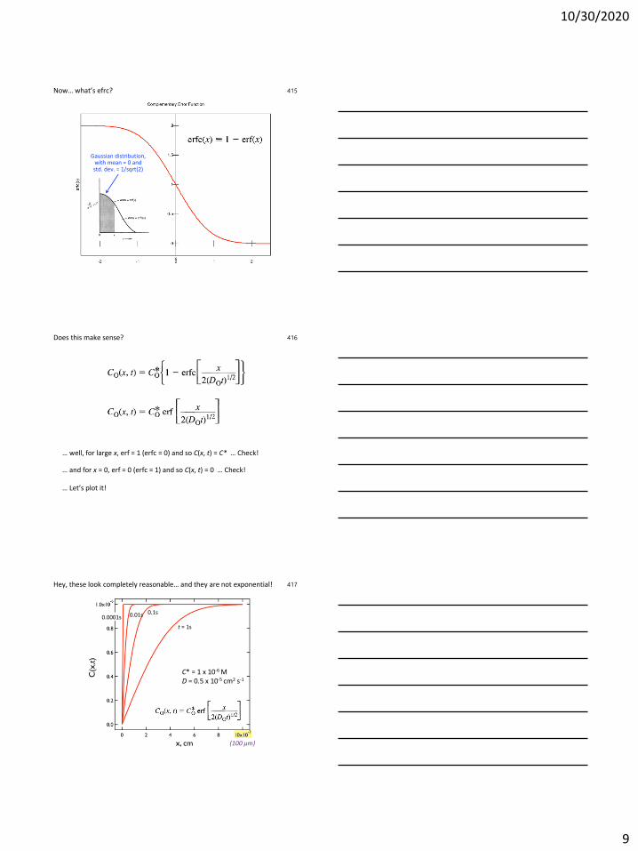
414What’s efrc?… Well, first of all, what’s the error function: erf?

10/30/2020

9

415Now… what’s efrc?

Gaussian distribution,with mean = 0 andstd. dev. = 1/sqrt(2)

416

… well, for large x, erf = 1 (erfc = 0) and so C(x, t) = C* … Check!

… and for x = 0, erf = 0 (erfc = 1) and so C(x, t) = 0 … Check!

… Let’s plot it!

Does this make sense?

417

C* = 1 x 10-6 MD = 0.5 x 10-5 cm2 s-1

t = 1s

0.1s0.01s

Hey, these look completely reasonable… and they are not exponential!

(100 µm)

0.0001s

10/30/2020

10

ഥΔ = 2𝑑 𝐷𝑡, where d is the dimension

… and the “2” is for positive and negative directions

418How large is the diffusion layer? Recall the rms displacement…

root mean square (rms) displacement(standard deviation)

Dimension Δ*=

1D

2D

3D

*the rms displacement

… plane

… wire, line, tube

… point, sphere, disk

a characteristic"diffusion length"

2𝐷𝑡

4𝐷𝑡

6𝐷𝑡

ഥΔ = 2𝑑 𝐷𝑡 =cm2

ss = cm

In both directions from a…

419

2.2 µm7.1 µm 22 µm

t = 1s

0.1s

Hey, these look completely reasonable for 1D diffusion in one direction!

0.01s0.0001s

… use the geometric area for calculations

C* = 1 x 10-6 MD = 0.5 x 10-5 cm2 s-1

𝐷𝑡 =(100 µm)

Why is 52% of thebulk concentrationnoteworthy?

Plug in x = (Dt)0.5!… Ah ha!

OK… that’s Step #1… Whoa! That was deep!… The last two steps are not… 420



i = nFAJO(0, t)


10/30/2020

11

421

… but we just derived CO(x, t):

… now Step #2…

(Fick’s First Law)

… and so we need to evaluate:

−𝐽O 𝑥, 𝑡 = 𝐷O𝜕

𝜕𝑥𝐶∗erf

𝑥

2 𝐷O𝑡

422

… we use the Leibniz rule, to get d/dx(erf(x)) as follows:

… now Step #2…

see B&F,pg. 780,for details

… and using this in conjunction with the chain rule, we get:

… and when x = 0 (at the electrode), we get:

−𝐽O 𝑥, 𝑡 = 𝐷O𝜕

𝜕𝑥𝐶∗erf

𝑥

2 𝐷𝑡

−𝐽O 0, 𝑡 = 𝐶∗𝐷O𝜋𝑡

−𝐽O 𝑥, 𝑡 = 𝐷O𝐶∗

1

2 𝐷O𝑡

2

𝜋exp

−𝑥2

4𝐷O𝑡

… which is what we needed for Step #3…

OK… that’s Steps #1 and 2… 423



i = nFAJO(0, t)


10/30/2020

12

424… and finally, Step #3 using Step #2…

the Cottrell Equation

Frederick Gardner Cottrell, in 1920b. January 10, 1877, Oakland, California, U.S.A.

d. November 16, 1948, Berkeley, California, U.S.A.

… established Research Corporation for Science Advancement in 1912

… initial funding from profits on patents for the electrostatic precipitator, used to clear smokestacks of charged soot particles

… and with i = nFAJO(0, t)…

−𝐽O 0, 𝑡 = 𝐶∗𝐷𝑂𝜋𝑡

425

http://en.wikipedia.org/wiki/Electrostatic_precipitatorhttp://en.wikipedia.org/wiki/Corona_discharge

> 1 kVneutral particles

corona dischargecapture plates

charged particles

Cottrell, then at UC Berkeley, invented the electrostatic precipitator usedto clear smokestacks of charged soot particles…

426

http://en.wikipedia.org/wiki/Electrostatic_precipitator

10/30/2020

13

427

D = 1.5 x 10-6 cm2 s-1

D = 1 x 10-5 cm2 s-1

… OK, so what does it predict?

(10 ms)

the Cottrell

Equation

428

D = 1.5 x 10-6 cm2 s-1

D = 1 x 10-5 cm2 s-1

… OK, so what does it predict?

(short time)(long time)

Plot data like thisonly for visualizationpurposes, and not forfitting the data as yourstatistics and thus best-fit values will beaffected and incorrect.

the Cottrell

Equation

429… OK, so what does it predict?

?????

(short time)(long time)

the Cottrell

Equation

slope =nFAπ -1/2D1/2C*

10/30/2020

14

430… use the Cottrell Equation to measure D, such as in thin films/coatings!… but what are the problems with this approach?

the integratedCottrell Equation

1) Huge initial currents… beware of compliance current!

2) Noise.

3) RC time limitations decrease expected current at really short times.

4) Roughness factor increases expected current at short times.

5) Adsorbed (electrolyzable) gunk increases expected current at short times.

6) Convection, “edge effects,” and thin pathlengths impose a “long” time

limit to these types of experiments.

… Solution: Integrate the Cottrell equation with respect to time…

the Cottrell

Equation

Date post:	27-Mar-2022
Category:	Documents
Upload:	others
View:	0 times
Download:	0 times

Lecture #12 of 26

Documents