37
Lecture 12 • One-way Analysis of Variance (Chapter 15.2) • Multiple comparisons for one- way ANOVA (Chapter 15.7)
| Date post: | 21-Dec-2015 |
| Category: |
Documents |
| View: | 231 times |
| Download: | 3 times |
Lecture 12
• One-way Analysis of Variance (Chapter 15.2)
• Multiple comparisons for one-way ANOVA (Chapter 15.7)

Review of one-way ANOVA
• Objective: Compare the means of K populations of interval data based on independent random samples from each.
• H0: • H1: At least two means differ• Notation: xij – ith observation of jth sample;
- mean of the jth sample; nj – number of observations in jth sample; - grand mean of all observations
K 21
jx
x

• The marketing manager for an apple juice manufacturer needs to
decide how to market a new product. Three strategies are considered,
which emphasize the convenience, quality and low price of product
respectively.
• An experiment was conducted as follows:
• In three cities an advertisement campaign was launched .
• In each city only one of the three characteristics (convenience,
quality, and price) was emphasized.
• The weekly sales were recorded for twenty weeks following
the beginning of the campaigns.
Example 15.1

Rationale Behind Test Statistic
• Two types of variability are employed when testing for the equality of population means– Variability of the sample means– Variability within samples
• Test statistic is essentially (Variability of the sample means)/(Variability within samples)
The rationale behind the test statistic – I
• If the null hypothesis is true, we would expect all the sample means to be close to one another (and as a result, close to the grand mean).
• If the alternative hypothesis is true, at least some of the sample means would differ.
• Thus, we measure variability between sample means.
• The variability between the sample means is measured as the sum of squared distances between each group mean and the grand mean times the sample size of the group.
This sum is called the
Sum of Squares for Treatments
SSTIn our example treatments arerepresented by the differentadvertising strategies.
Variability between sample means
2k
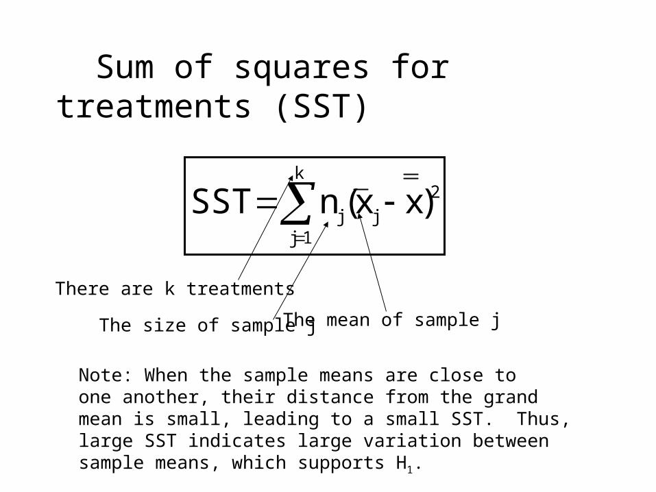
1jjj )xx(nSST
There are k treatments
The size of sample j The mean of sample j
Sum of squares for treatments (SST)
Note: When the sample means are close toone another, their distance from the grand mean is small, leading to a small SST. Thus, large SST indicates large variation between sample means, which supports H1.

• Solution – continuedCalculate SST
2k
1jjj
321
)xx(nSST
65.608x00.653x577.55x
= 20(577.55 - 613.07)2 + + 20(653.00 - 613.07)2 + + 20(608.65 - 613.07)2 == 57,512.23
The grand mean is calculated by
k21
kk2211
n...nnxn...xnxn
X
Sum of squares for treatments (SST)

Is SST = 57,512.23 large enough to reject H0 in favor of H1?
Large compared to what?
Sum of squares for treatments (SST)

20
25
30
1
7
Treatment 1 Treatment 2 Treatment 3
10
12
19
9
Treatment 1Treatment 2Treatment 3
20
161514
1110
9
10x1
15x2
20x3
10x1
15x2
20x3
The sample means are the same as before,but the larger within-sample variability makes it harder to draw a conclusionabout the population means.
A small variability withinthe samples makes it easierto draw a conclusion about the population means.

• Large variability within the samples weakens the “ability” of the sample means to represent their corresponding population means.
• Therefore, even though sample means may markedly differ from one another, SST must be judged relative to the “within samples variability”.
The rationale behind test statistic – II

• The variability within samples is measured by adding all the squared distances between observations and their sample means.
This sum is called the
Sum of Squares for Error
SSEIn our example this is the sum of all squared differencesbetween sales in city j and thesample mean of city j (over all the three cities).
Within samples variability

• Solution – continuedCalculate SSE
Sum of squares for errors (SSE)
k
jjij
n
i
xxSSE
sss
j
1
2
1
23
22
21
)(
24.670,811,238,700.775,10
(n1 - 1)s12 + (n2 -1)s2
2 + (n3 -1)s32
= (20 -1)10,774.44 + (20 -1)7,238.61+ (20-1)8,670.24 = 506,983.50

Is SST = 57,512.23 large enough relative to SSE = 506,983.50 to reject the null hypothesis that specifies that all the means are equal?
Sum of squares for errors (SSE)

To perform the test we need to calculate the mean squaresmean squares as follows:
The mean sum of squares
Calculation of MST - Mean Square for Treatments
12.756,2813
23.512,571
k
SSTMST
Calculation of MSEMean Square for Error
45.894,8360
50.983,509
kn
SSEMSE

And finally the hypothesis test:
H0: 1 = 2 = …=k
H1: At least two means differ
Test statistic:
R.R: F>F,k-1,n-k
MSEMST
F
The F test rejection region

The F test
Ho: 1 = 2= 3
H1: At least two means differ
Test statistic F= MST MSE= 3.2315.3FFF:.R.R 360,13,05.0knk 1
Since 3.23 > 3.15, there is sufficient evidence to reject Ho in favor of H1, and argue that at least one of the mean sales is different than the others.
23.317.894,812.756,28
MSEMST
F
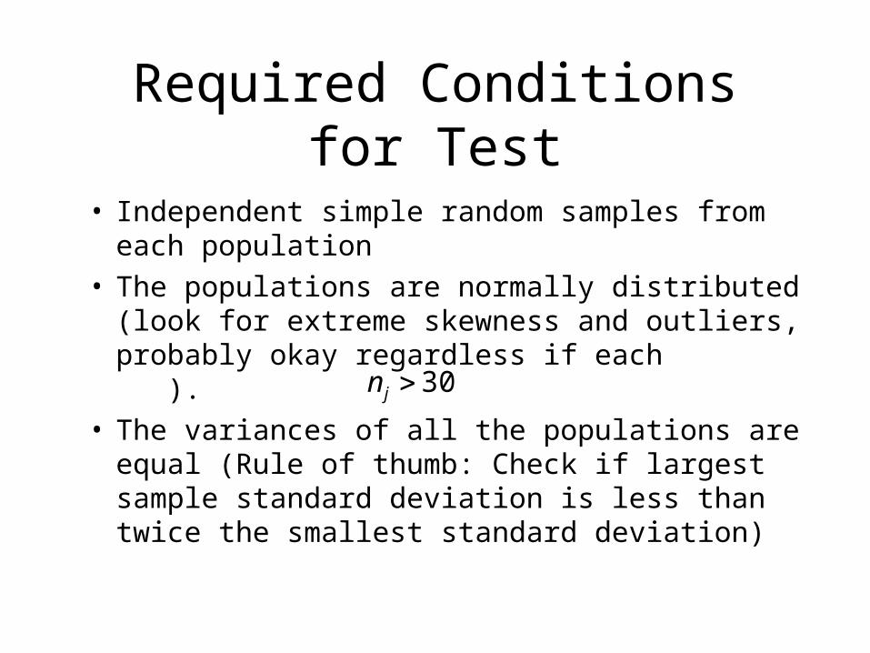
Required Conditions for Test
• Independent simple random samples from each population
• The populations are normally distributed (look for extreme skewness and outliers, probably okay regardless if each ).
• The variances of all the populations are equal (Rule of thumb: Check if largest sample standard deviation is less than twice the smallest standard deviation)
30jn

ANOVA Table – Example 15.1Analysis of Variance
Source DF Sum of Squares
Mean Square
F Ratio Prob > F
City 2 57512.23 28756.1 3.2330 0.0468
Error 57 506983.50 8894.4
C. Total
59 564495.73

Model for ANOVA
• = ith observation of jth sample• • is the overall mean level, is the differential
effect of the jth treatment and is the random error in the ith observation under the jth treatment. The errors are assumed to be independent, normally distributed with mean zero and variance The are normalized:
ijX
ijjijX
j
ij
2
j
K
j j10
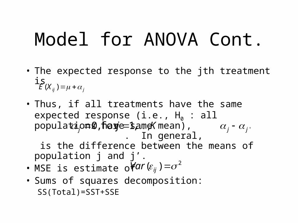
Model for ANOVA Cont.
• The expected response to the jth treatment is
• Thus, if all treatments have the same expected response (i.e., H0 : all populations have same mean), . In general, is the difference between the means of population j and j’.
• MSE is estimate of • Sums of squares decomposition:
SS(Total)=SST+SSE
jijXE )(
Kjj ,,1for ,0 'jj
2)( ijVar

Review Question: Intro to ANOVA
• Which case does ANOVA generalize?– 2-sample mean comparison with equal variance
assumption– 2-sample mean comparison with unequal variances
permitted– 2-sample variance comparison

Relationship between F-test and t-test for two samples
• For comparing two samples, the F-statistic equals the square of the t-statistic with equal variances.
• For two samples, the ANOVA F-test is equivalent to testing versus .
210 : H
211 : H
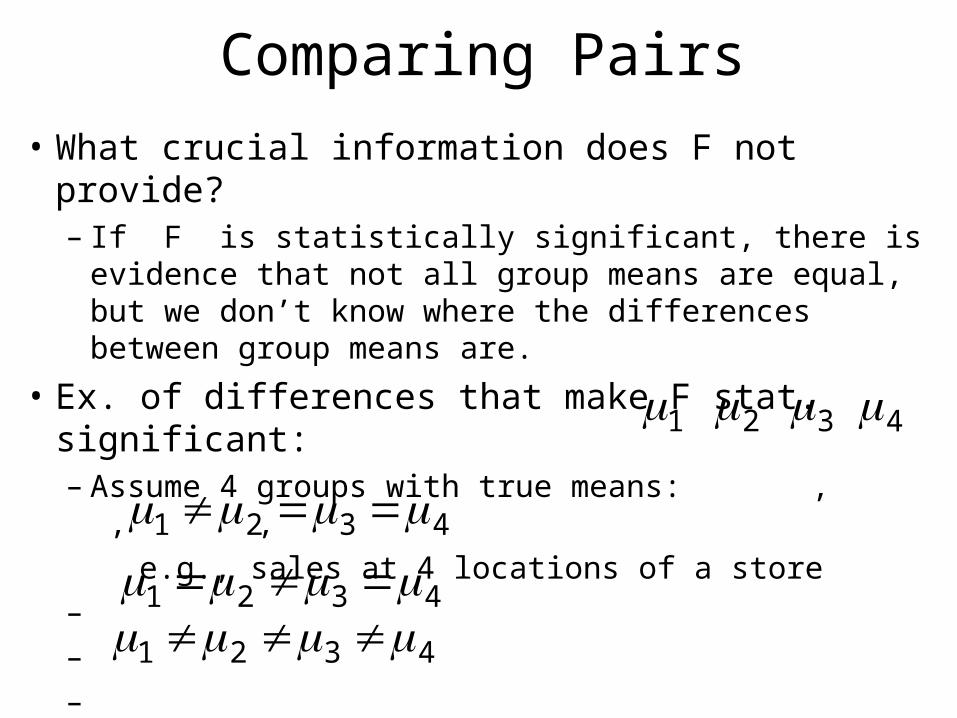
Comparing Pairs
• What crucial information does F not provide?– If F is statistically significant, there is evidence that
not all group means are equal, but we don’t know where the differences between group means are.
• Ex. of differences that make F stat. significant:– Assume 4 groups with true means: , , ,
e.g., sales at 4 locations of a store– – –
1 2 3 4
4321
4321 4321
15.7 Multiple Comparisons
• When the null hypothesis is rejected, it may be desirable to find which mean(s) is (are) different, and at how they rank.
• Three statistical inference procedures, geared at doing this, are presented:– Fisher’s least significant difference (LSD) method
– Bonferroni adjustment to Fisher’s LSD
– Tukey’s multiple comparison method
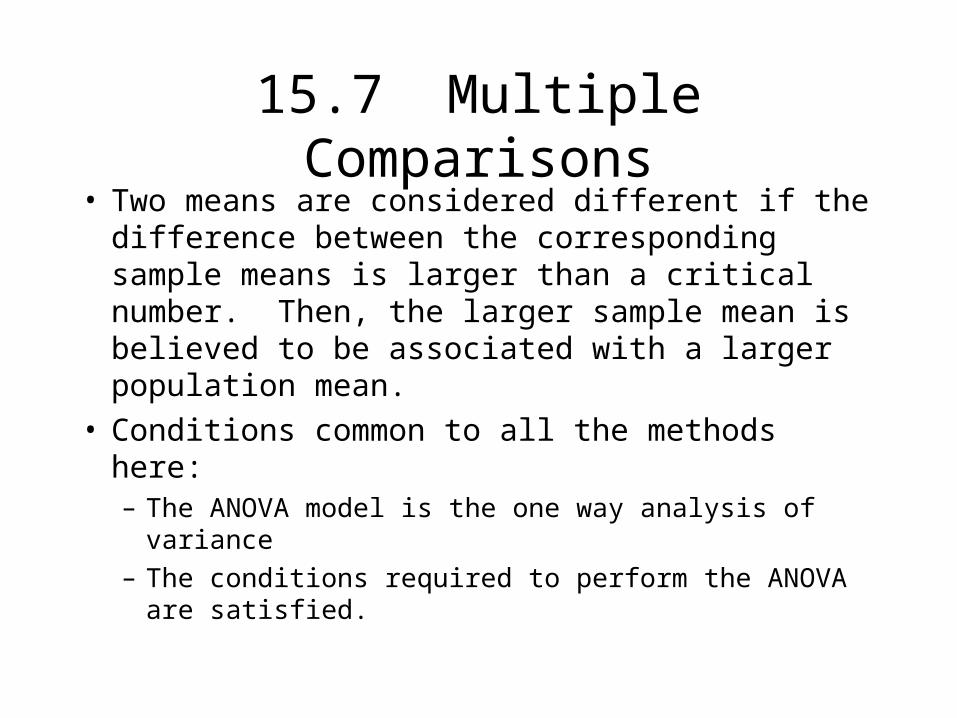
• Two means are considered different if the difference between the corresponding sample means is larger than a critical number. Then, the larger sample mean is believed to be associated with a larger population mean.
• Conditions common to all the methods here:– The ANOVA model is the one way analysis of variance
– The conditions required to perform the ANOVA are satisfied.
15.7 Multiple Comparisons

Fisher Least Significant Different (LSD) Method
• This method builds on the equal variances t-test of the difference between two means.
• The test statistic is improved by using MSE rather than sp
2.• We conclude that i and j differ (at % significance
level if > LSD, where
)11
(,2ji
kn nnMSEtLSD
|| ji xx

Experimentwise Type I error rate (E)(the effective Type I error)
• Using Fisher’s method may result in an increased probability of committing a type I error.
• The experimentwise Type I error rate is the probability of committing at least one Type I error at significance level of If C independent tests are done,
E = 1-(1 – )C
• The Bonferroni adjustment determines the required Type I error probability per test () , to secure a pre-determined overall E

Multiple Comparisons Problem
• A hypothetical study of the effect of birth control pills is done.
• Two groups of women (one taking birth controls, the other not) are followed and 100 variables are recorded for each subject such as blood pressure, psychological and medical problems.
• After the study, two-sample t-tests are performed for each variable and it is found that women taking birth pills have higher incidences of depression at the 5% significance level (the p-value equals .02).
• Does this provide strong evidence that women taking birth control pills are more likely to be depressed?
Bonferroni Adjustment
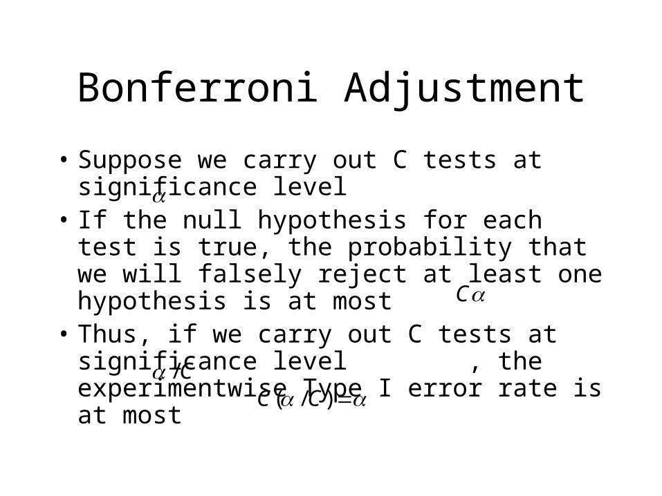
• Suppose we carry out C tests at significance level
• If the null hypothesis for each test is true, the probability that we will falsely reject at least one hypothesis is at most
• Thus, if we carry out C tests at significance level , the experimentwise Type I error rate is at most
C
C/ )/( CC

• The procedure:– Compute the number of pairwise comparisons (C)
[all: C=k(k-1)/2], where k is the number of populations.
– Set = E/C, where E is the true probability of making at least one Type I error (called experimentwise Type I error).
– We conclude that i and j differ at /C% significance level (experimentwise error rate at most )
)11
(),2(ji
knCji nnMSEt
Bonferroni Adjustment for ANOVA

35.4465.6080.653xx
10.3165.60855.577xx
45.750.65355.577xx
32
31
21
• Example 15.1 - continued
– Rank the effectiveness of the marketing strategies(based on mean weekly sales).
– Use the Fisher’s method, and the Bonferroni adjustment method
• Solution (the Fisher’s method)
– The sample mean sales were 577.55, 653.0, 608.65.
– Then,
71.59)20/1()20/1(8894
)11
(
57,2/05.
,2
t
nnMSEt
jikn
Fisher and Bonferroni Methods

• Solution (the Bonferroni adjustment)– We calculate C=k(k-1)/2 to be 3(2)/2 = 3.
– We set = .05/3 = .0167, thus t.01672, 60-3 = 2.467 (Excel).
54.73)20/1()20/1(8894467.2
)n1
n1
(MSEtji
2
Again, the significant difference is between 1 and 2.
35.4465.6080.653xx
10.3165.60855.577xx
45.750.65355.577xx
32
31
21
Fisher and Bonferroni Methods

• The test procedure: – Assumes equal number of obs. per populations.– Find a critical number as follows:
gnMSE
),k(q
k = the number of populations =degrees of freedom = n - kng = number of observations per population = significance levelq(k,) = a critical value obtained from the studentized range table (app. B17/18)
Tukey Multiple Comparisons

If the sample sizes are not extremely different, we can use the above procedure with ng calculated as the harmonic mean ofthe sample sizes. k21 n1...n1n1
kgn
• Repeat this procedure for each pair of samples. Rank the means if possible.
• Select a pair of means. Calculate the difference between the larger and the smaller mean.
• If there is sufficient evidence to conclude that max > min .
minmax xx
minmax xx
Tukey Multiple Comparisons
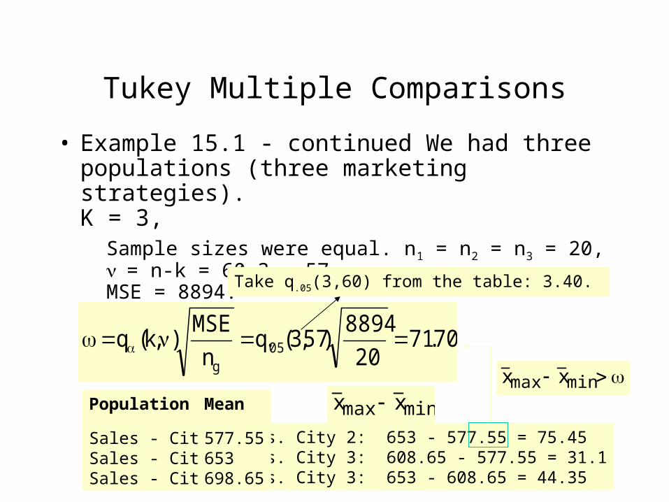
City 1 vs. City 2: 653 - 577.55 = 75.45City 1 vs. City 3: 608.65 - 577.55 = 31.1City 2 vs. City 3: 653 - 608.65 = 44.35
• Example 15.1 - continued We had three populations (three marketing strategies).K = 3,
Sample sizes were equal. n1 = n2 = n3 = 20,= n-k = 60-3 = 57,MSE = 8894.
minmax xx
70.7120
8894)57,3(.q
nMSE
),k(q 05g
Take q.05(3,60) from the table: 3.40.
Population
Sales - City 1Sales - City 2Sales - City 3
Mean
577.55653698.65
minmax xx
Tukey Multiple Comparisons

Practice Problems
• 15.16, 15.22, 15.26, 15.66


