Lecture 14

• Analysis of Variance Experimental Designs (Chapter 15.3)

• Randomized Block (Two-Way) Analysis of Variance

• Announcement: Extra office hours, today after class and Monday, 9:00-10:20

15.3 Analysis of Variance Experimental Designs

• Several elements may distinguish between one experimental design and another:– The number of factors (1-way, 2-way, 3-way,…

ANOVA).– The number of factor levels.– Independent samples vs. randomized blocks– Fixed vs. random effects

These concepts will be explained in this lecture.

Number of factors, levels• Example: 15.1, modified

– Methods of marketing: price, convenience, quality => first factor with 3 levels

– Medium: advertise on TV vs. in newspapers => second factor with 2 levels

• This is a factorial experiment with two “crossed factors” if all 6 possibilities are sampled or experimented with.

• It will be analyzed with a “2-way ANOVA”. (The book got this term wrong.)

Factor ALevel 1Level2

Level 1

Factor B

Level 3

Two - way ANOVATwo factors

Level2

One - way ANOVASingle factor

Treatment 3 (level 1)

Response

Response

Treatment 1 (level 3)

Treatment 2 (level 2)

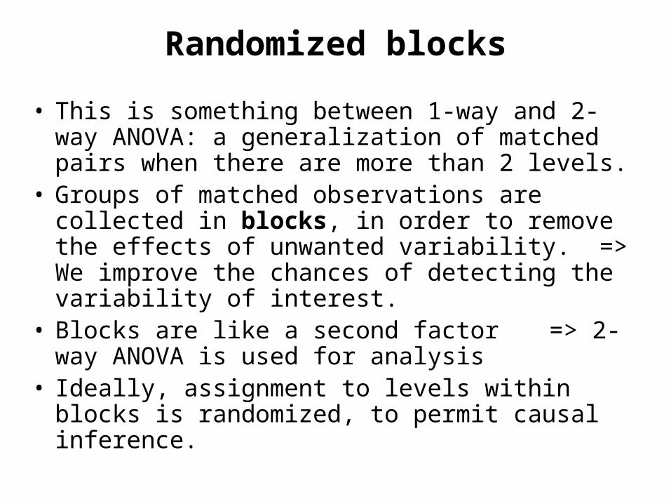
• This is something between 1-way and 2-way ANOVA: a generalization of matched pairs when there are more than 2 levels.

• Groups of matched observations are collected in blocks, in order to remove the effects of unwanted variability. => We improve the chances of detecting the variability of interest.

• Blocks are like a second factor => 2-way ANOVA is used for analysis

• Ideally, assignment to levels within blocks is randomized, to permit causal inference.

Randomized blocks

Randomized blocks (cont.)• Example: expand 13.03

– Starting salaries of marketing and finance MBAs: add accounting MBAs to the investigation.

– If 3 independent samples of each specialty are collected (samples possibly of different sizes), we have a 1-way ANOVA situation with 3 levels.

– If GPA brackets are formed, and if one samples 3 MBAs per bracket, one from each specialty, then one has a blocked design. (Note: the 3 samples will be of equal size due to blocking.)

– Randomization is not possible here: one can’t assign each student to a specialty

=> No causal inference.

• Fixed effects– If all possible levels of a factor are included in our

analysis or the levels are chosen in a nonrandom way, we have a fixed effect ANOVA.

– The conclusion of a fixed effect ANOVA applies only to the levels studied.

• Random effects– If the levels included in our analysis represent a random

sample of all the possible levels, we have a random-effect ANOVA.

– The conclusion of the random-effect ANOVA applies to all the levels (not only those studied).

Models of fixed and random effects

Fixed and random effects - examples– Fixed effects - The advertisement Example (15.1): All

the levels of the marketing strategies considered were included. Inferences don’t apply to other possible strategies such as emphasizing nutritional value.

– Random effects - To determine if there is a difference in the production rate of 50 machines in a large factory, four machines are randomly selected and the number of units each produces per day for 10 days is recorded.

Models of fixed and random effects (cont.)

15.4 Randomized Blocks Analysis of Variance

• The purpose of designing a randomized block experiment is to reduce the within-treatments variation, thus increasing the relative amount of between treatment variation.

• This helps in detecting differences between the treatment means more easily.

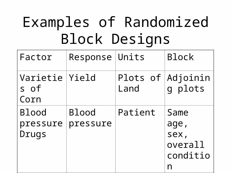
Examples of Randomized Block Designs

Factor Response Units Block

Varieties of Corn

Yield Plots of Land

Adjoining plots

Blood pressure Drugs

Blood pressure

Patient Same age, sex, overall condition

Number of breaks

Worker productivity

Worker Shifts

Treatment 4

Treatment 3

Treatment 2

Treatment 1

Block 1Block3 Block2

Block all the observations with some commonality across treatments

Randomized Blocks

TreatmentBlock 1 2 k Block mean

1 X11 X12 . . . X1k2 X21 X22 X2k...b Xb1 Xb2 Xbk

Treatment mean

1]B[x

2]B[x

b]B[x

1]T[x 2]T[x k]T[x

Block all the observations with some commonality across treatments

Randomized Blocks

• The sum of square total is partitioned into three sources of variation– Treatments– Blocks– Within samples (Error)

SS(Total) = SST + SSB + SSESS(Total) = SST + SSB + SSE

Sum of square for treatments Sum of square for blocks Sum of square for error

Recall. For the independent samples design we have: SS(Total) = SST + SSE

Partitioning the total variability

Sums of Squares Decomposition

• = observation in ith block, jth treatment

• = mean of ith block

• = mean of jth treatment

•

ijX

iX

jX

k

j

b

ijiij

b

ii

k

jj

k

j

b

iij

XXXXSSBSSTSSTotSSE

XXkSSB

XXbSST

XXSSTot

1 1

2

2

1

1

2

1 1

2

)(

)(

)(

)(

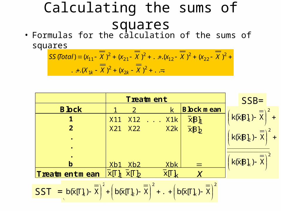
Calculating the sums of squares• Formulas for the calculation of the sums of squares

TreatmentBlock 1 2 k Block mean

1 X11 X12 . . . X1k2 X21 X22 X2k...b Xb1 Xb2 Xbk

Treatment mean

1]B[x

2]B[x

1]T[x 2]T[x k]T[x x2

1 X)]T[x(b

...X)]T[x(b

2

2

2

k X)]T[x(b

SST =

2

1 X)]B[x(k

2

2 X)]B[x(k

2

k X)]B[x(k

SSB=

...)()(...

)()(...)()()(

22

21

222

212

221

211

XxXX

XxXxXxXxTotalSS

kk

Calculating the sums of squares• Formulas for the calculation of the sums of squares

TreatmentBlock 1 2 k Block mean

1 X11 X12 . . . X1k2 X21 X22 X2k...b Xb1 Xb2 Xbk

Treatment mean

1]B[x

2]B[x

1]T[x 2]T[x k]T[x x2

1 X)]T[x(b

...X)]T[x(b

2

2

2

k X)]T[x(b

SST =

2

1 X)]B[x(k

2

2 X)]B[x(k

2

k X)]B[x(k

SSB=

...)X]B[x]T[xx()X]B[x]T[xx(

...)X]B[x]T[xx()X]B[x]T[xx(

...)X]B[x]T[xx()X]B[x]T[xx(SSE

22kk2

21kk1

22222

21212

22121

21111

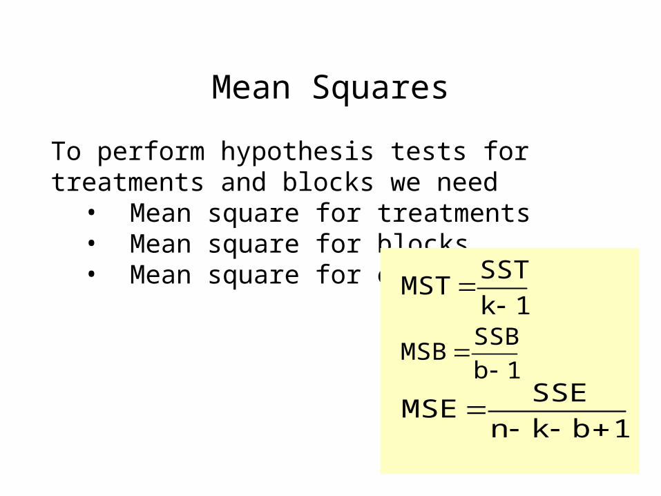
To perform hypothesis tests for treatments and blocks we need

• Mean square for treatments• Mean square for blocks• Mean square for error

Mean Squares

1kSST

MST

1bSSB

MSB

1bknSSE

MSE

Test statistics for the randomized block design ANOVA

MSEMST

F

MSEMSB

F

Test statistic for treatments

Test statistic for blocks

df-T: k-1 df-B: b-1 df-E: n-k-b+1

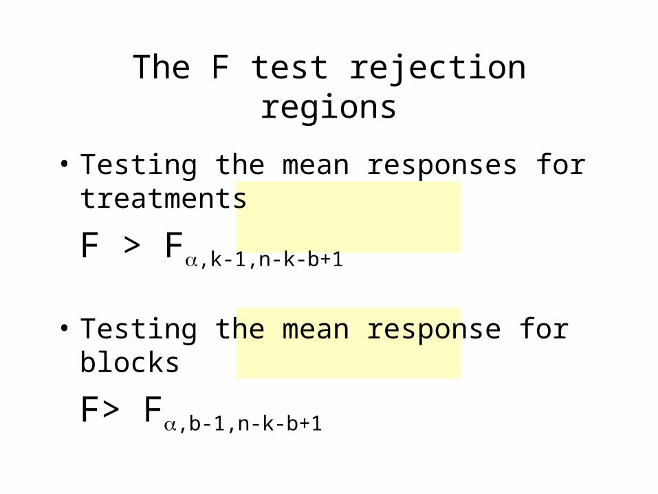
• Testing the mean responses for treatments

F > F,k-1,n-k-b+1

• Testing the mean response for blocks

F> F,b-1,n-k-b+1

The F test rejection regions

• Example 15.2– Are there differences in the effectiveness of

cholesterol reduction drugs? – To answer this question the following experiment

was organized:• 25 groups of men with high cholesterol were matched by

age and weight. Each group consisted of 4 men.• Each person in a group received a different drug.• The cholesterol level reduction in two months was

recorded.

– Can we infer from the data in Xm15-02 that there are differences in mean cholesterol reduction among the four drugs?

Randomized Blocks ANOVA - Example

• Solution– Each drug can be considered a treatment.

– Each 4 records (per group) can be blocked, because they are matched by age and weight.

– This procedure eliminates the variability in cholesterol reduction related to different combinations of age and weight.

– This helps detect differences in the mean cholesterol reduction attributed to the different drugs.

Randomized Blocks ANOVA - Example

BlocksTreatments b-1 MST / MSE MSB / MSE

Conclusion: At 5% significance level there is sufficient evidence to infer that the mean “cholesterol reduction” gained by at least two drugs are different.

K-1

Randomized Blocks ANOVA - Example

ANOVASource of Variation SS df MS F P-value F critRows 3848.7 24 160.36 10.11 0.0000 1.67Columns 196.0 3 65.32 4.12 0.0094 2.73Error 1142.6 72 15.87

Total 5187.2 99

Required Conditions for Test

• The sample from each block in each population is a simple random sample from the block in that population

• There are conditions that are similar to the populations being normal and having equal variance but they are more complicated (the book’s description is wrong). We shall discuss this more when we cover regression. For now, you should just look for outliers.

Criteria for Blocking

• Goal is to find criteria for blocking that significantly affect the response variable

• Effect of teaching methods on student test scores.– Good blocking variable: GPA– Bad blocking variable: Hair color

• Ideal design of experiment is often to make each subject a block and apply the entire set of treatments to each subject (e.g., give different drugs to each subject) but not always physically possible.

Test of whether blocking is effective

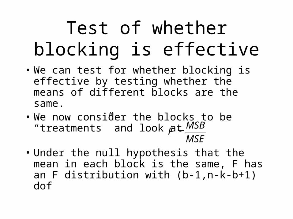
• We can test for whether blocking is effective by testing whether the means of different blocks are the same.

• We now consider the blocks to be “treatments” and look at

• Under the null hypothesis that the mean in each block is the same, F has an F distribution with (b-1,n-k-b+1) dof

MSE

MSBF

Practice Problems

• 15.38, 15.40