Shocks to aggregate demand and aggregate supply

Lecture 16

October 27th, 2017

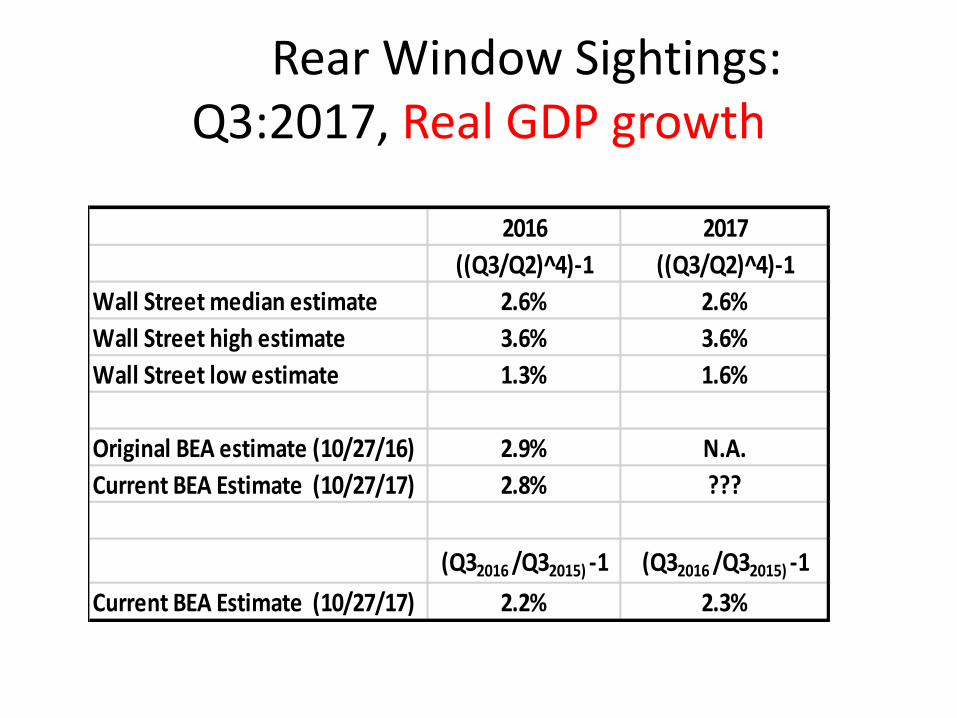
Rear Window Sightings:Q3:2017, Real GDP growth

2016 2017

((Q3/Q2)^4)-1 ((Q3/Q2)^4)-1

Wall Street median estimate 2.6% 2.6%

Wall Street high estimate 3.6% 3.6%

Wall Street low estimate 1.3% 1.6%

Original BEA estimate (10/27/16) 2.9% N.A.

Current BEA Estimate (10/27/17) 2.8% ???

(Q32016 /Q32015) -1 (Q32016 /Q32015) -1

Current BEA Estimate (10/27/17) 2.2% 2.3%

Atlanta Fed NowCast, as of 10/26versus BEA estimate, as of 10/27:

Atlanta Fed Atlanta Fed BEA BEA

((Q3/Q2)^4)-1 Q3/Q2 percentage ((Q3/Q2)^4)-1 Q3/Q2 percentage

(percent) contribution (percent) contribution

(percentage points)

Y, Real GDP 2.5% 2.5 3.00% 3

C 2.5% 1.7 2.40% 1.6

C, motor vehicles

I

I, housing -3.6% -0.14 -6.00% -0.24

I, equipment 5.6% 0.51 6.00% 0.61

I, inventories N.A. 0.80 0.73

G -1.7% -0.30 -0.10% 0

NX, net exports 0.07 0.41

X, exports 2.5% 2.30%

M, Imports 1.6% -0.80%

Characterizing Changes in Values for key variables as Shocks

• Why Call Them Shocks?

• Most economic models are

EQUILIBRIUM SEEKING

• When something occurs outside of the forces that drive the model it SHOCKS system and the model pushes toward a different equilibrium

Types of AD Shocks:Changes in variables that determine the position of the AD curve.

Δ Household expectations → Δ autonomous C (Δ ҧ𝐶)

Δ Personal taxes → Δ Yd → Δ C

Δ Profit expectations → Δ Investment = ҧ𝐼

Δ Interest Rates lead to Δ Investment = ҧ𝐼

Types of AS ShocksChanges in variables that determine the position of the AS curve.

Wages = W0

Productivity = Z0

Capital Stock = K0

Resource Prices = RP0

7 of 47© 2013 Pearson Education, Inc. Publishing as Prentice Hall

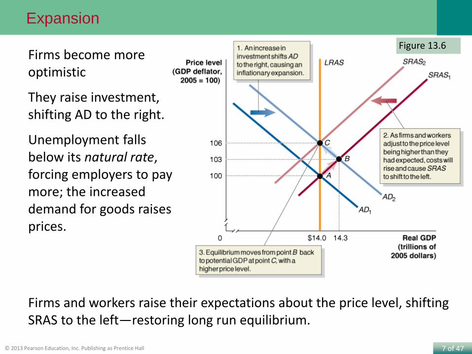
Figure 13.6

Expansion

Firms become more optimistic

They raise investment, shifting AD to the right.

Unemployment falls below its natural rate, forcing employers to pay more; the increased demand for goods raises prices.

Firms and workers raise their expectations about the price level, shifting SRAS to the left—restoring long run equilibrium.

8 of 47© 2013 Pearson Education, Inc. Publishing as Prentice Hall

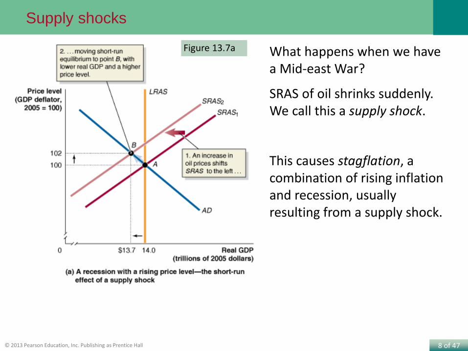
Figure 13.7a

Supply shocks

What happens when we have a Mid-east War?

SRAS of oil shrinks suddenly. We call this a supply shock.

This causes stagflation, a combination of rising inflation and recession, usually resulting from a supply shock.

9 of 47© 2013 Pearson Education, Inc. Publishing as Prentice Hall

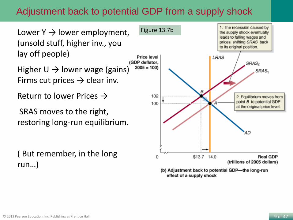
Figure 13.7b

Adjustment back to potential GDP from a supply shock

Lower Y → lower employment, (unsold stuff, higher inv., you lay off people)

Higher U → lower wage (gains) Firms cut prices → clear inv.

Return to lower Prices →

SRAS moves to the right, restoring long-run equilibrium.

( But remember, in the long run…)

A positive demand shock may be a mixed blessing

Dynamic interpretation:(How policy makers, CEO’s think about it)

• Few focus on the price level, or the level of GDP

•Δ𝑃

Δ𝑡= π The world watches the inflation rate.

More specifically:

•ΔπΔ𝑡

= The change in the pace of price changes.

•Δ𝑌

Δ𝑡= ሶ𝑌 ሶ𝑌 = real growth rate for the economy

• A Positive demand Shock:

π accelerates ሶ𝑌 accelerates

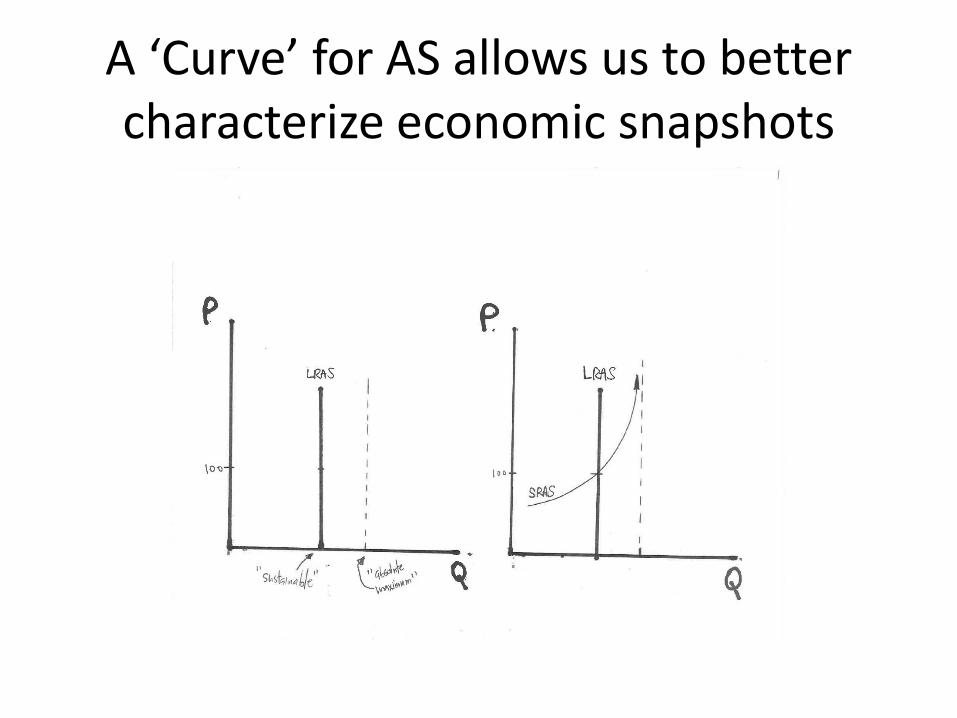
A ‘Curve’ for AS allows us to better characterize economic snapshots

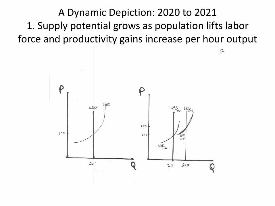
A Dynamic Depiction: 2020 to 20211. Supply potential grows as population lifts labor

force and productivity gains increase per hour output

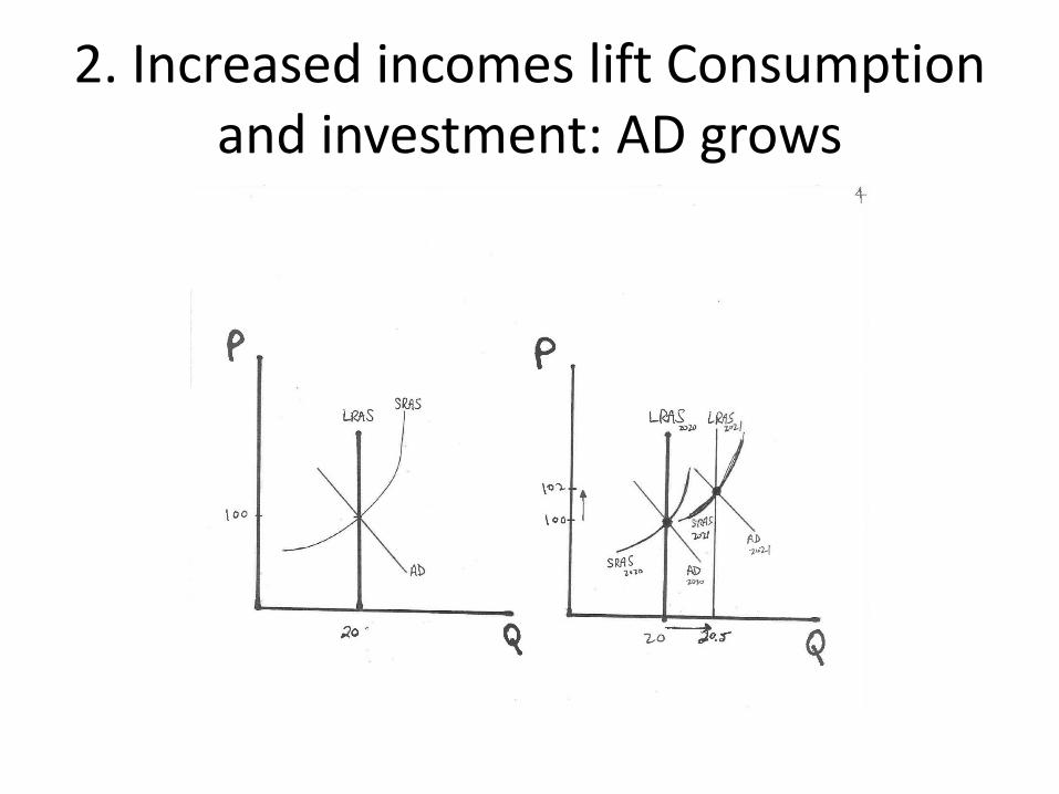
2. Increased incomes lift Consumption and investment: AD grows

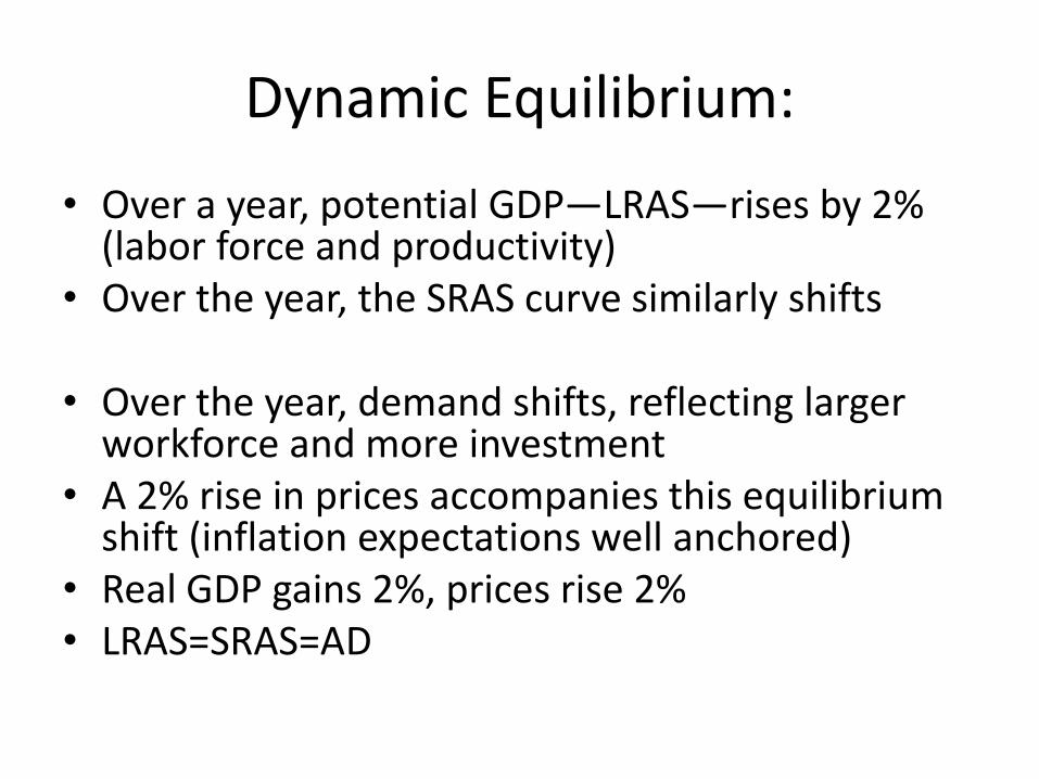
Dynamic Equilibrium:

• Over a year, potential GDP—LRAS—rises by 2% (labor force and productivity)

• Over the year, the SRAS curve similarly shifts

• Over the year, demand shifts, reflecting larger workforce and more investment

• A 2% rise in prices accompanies this equilibrium shift (inflation expectations well anchored)

• Real GDP gains 2%, prices rise 2% • LRAS=SRAS=AD

Shocks deliver what?

• The effects of demand and supply shocks depend, in part on the state of the economy before the shock.

• With high U and ample capacity, the supply curve is flattish.

• With very low U and little room to grow, the supply curve is very steep.

With ample excess capacity, a positive demand shocklifts output meaningfully and does little to prices

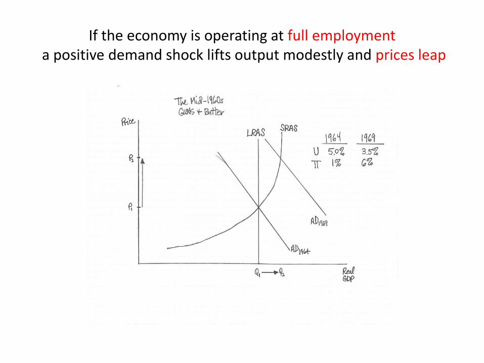
If the economy is operating at full employmenta positive demand shock lifts output modestly and prices leap

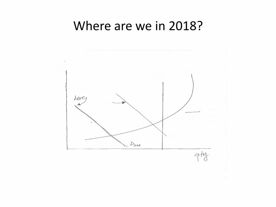
Where are we in 2018?

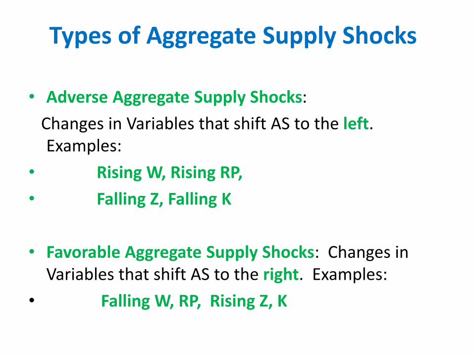
Types of Aggregate Supply Shocks

• Adverse Aggregate Supply Shocks:

Changes in Variables that shift AS to the left. Examples:

• Rising W, Rising RP,

• Falling Z, Falling K

• Favorable Aggregate Supply Shocks: Changes in Variables that shift AS to the right. Examples:

• Falling W, RP, Rising Z, K

A positive productivity shock:(The best news for the long run)

• Technology inventions lay the groundwork

• Explosive investment drives I0• Productivity, we shift people to new

endeavors

• That means we have more output, at a given price level

• AS shifts to the rightPrices Fall

Output Rises

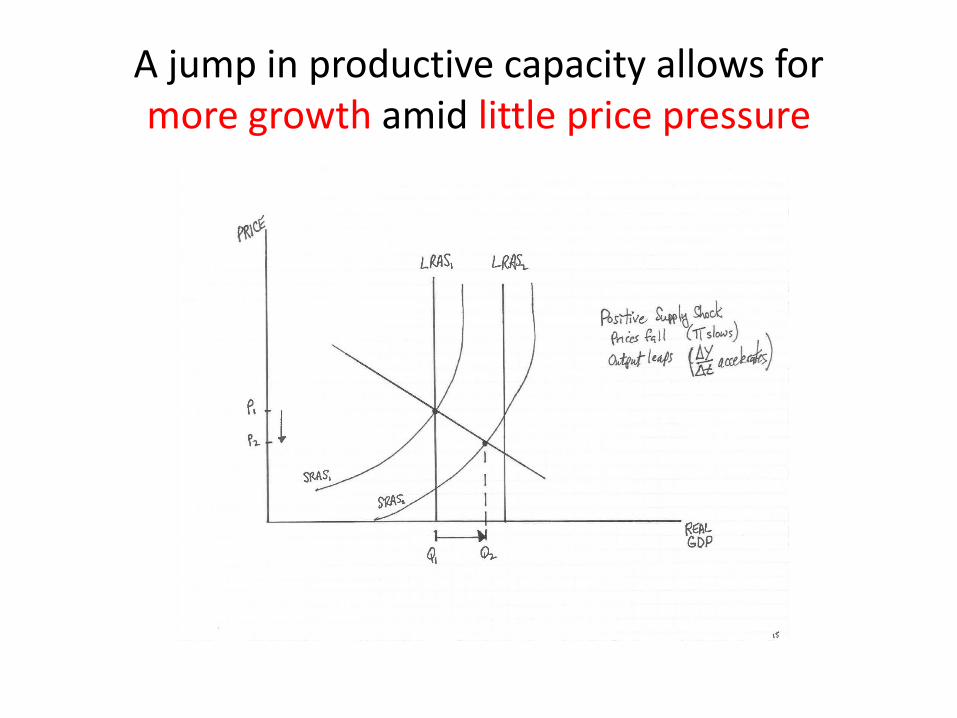
A jump in productive capacity allows for more growth amid little price pressure

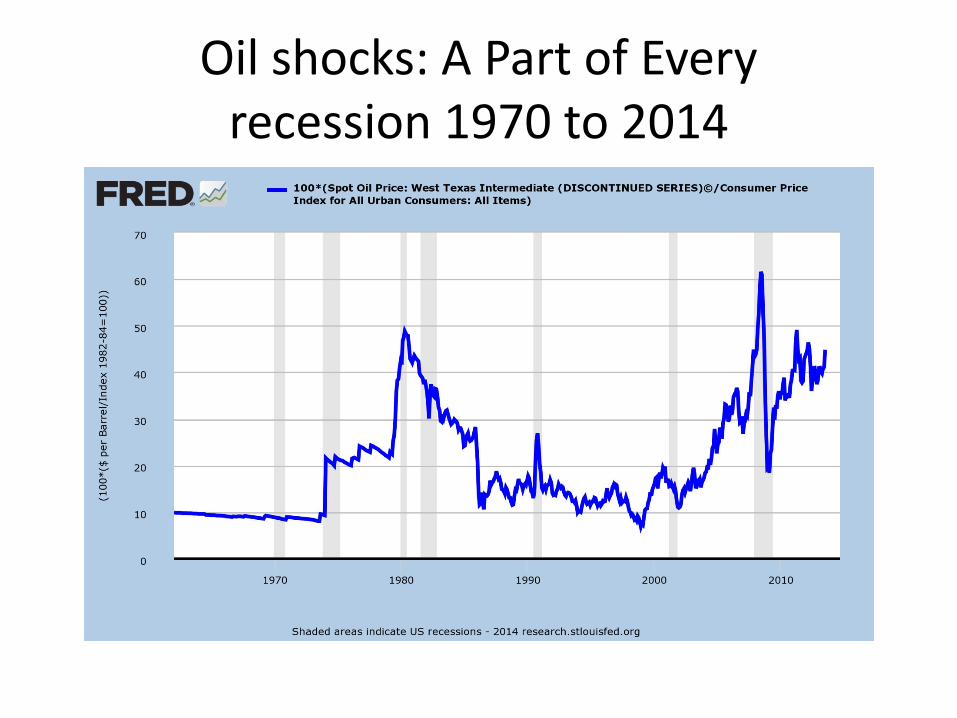
Oil shocks: A Part of Every recession 1970 to 2014

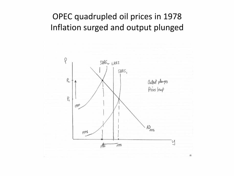
OPEC quadrupled oil prices in 1978Inflation surged and output plunged

AS Shocks: Equilibrium Price and Output move in opposite directions

• A Positive Supply Shock: (Surge in labor force)

Prices Fall

Output Rises

• An adverse supply shock: (Oil prices surge)

Prices Rise

Output Falls

The Great Recession/RecoveryA Three Part Story

• Act I: Q2:2007 to Q2:2008 – A standard adverse Supply Shock as Oil Prices surge

• Act II: Q2:2008 to Q2:2009 – An Adverse Demand Shock as interest rates surge and

consumer and business confidence plunge.

• Act III: Q2:2009 to Q2:2010– A Positive Demand Reversal as government spending

jumps, confidence rises and interest rates fall.

The bare facts of the three year swing for output and inflation:

REAL GDP 4-QTR CPI INDEX 4-QTR Potential 4-QTR

($ BILLIONS) CHANGE (LEVEL) CHANGE GDP CHANGE

Q2:2007 14,839 102.5 2.5% 14,800

Q2:2008 14,963 0.8% 106.6 4.0% 15,170 2.5%

Q2:2009 14,356 -4.1% 107.5 0.8% 15,473 2.0%

Q2:2010 14,746 2.7% 108.7 1.2% 15,783 2.0%

Act I:Oil Prices surge.A Negative SRAS Shock

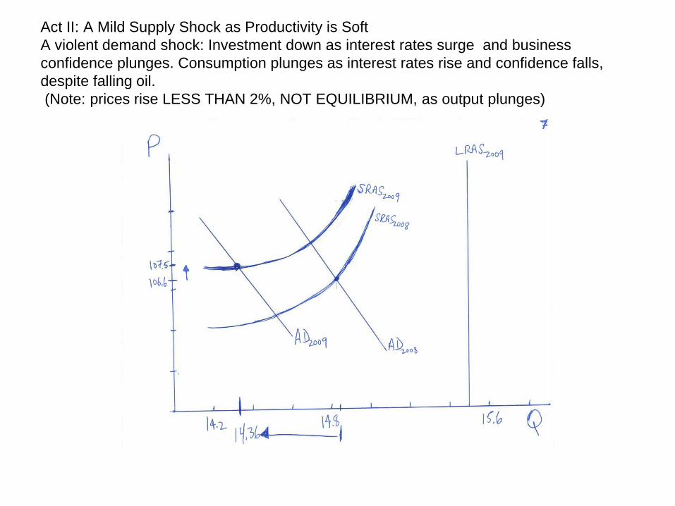
Act II: A Mild Supply Shock as Productivity is Soft

A violent demand shock: Investment down as interest rates surge and business

confidence plunges. Consumption plunges as interest rates rise and confidence falls,

despite falling oil.

(Note: prices rise LESS THAN 2%, NOT EQUILIBRIUM, as output plunges)

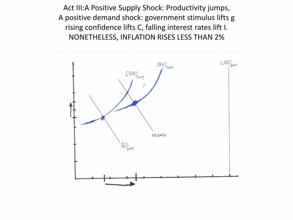
Act III:A Positive Supply Shock: Productivity jumps, A positive demand shock: government stimulus lifts g

rising confidence lifts C, falling interest rates lift I.NONETHELESS, INFLATION RISES LESS THAN 2%

THINGS TO PONDERABOUT 2010

• Why did inflation rise less than 2% despite aggressive government fiscal stimulus?

• Why did risky interest rates fall despite an explosive increase in government borrowing?

• Why did confidence rise despite an explosive rise in the size of the U.S. budget deficit?

• Why did I draw the SRAS curve ‘very flat’?

• Despite stimulus, where is GDP vs potential?

The 1990s technology boom

• Technology companies connect the phone and the computer

• GPS

• Cash machines

• Personal airline check in

• Phone help lines in India

The View in 1993

• We assumed the USA underlying inflation rate was a bit less than 3% in the early 1990s:1993 CPI YOY change = 2.7%

1994 CPI YOY change = 2.7%

• We assumed the USA underlying real GDP growth rate was a bit less than 3% in the early 1990s:1993 real GDP growth = 2.7%

The View in 1998

• We assumed the USA underlying inflation rate was below 2% in the late 1990s:1997 CPI YOY change = 1.7%

1998 CPI YOY change = 1.6%

• We assumed the USA underlying real GDP growth rate was above 4% in the late 1990s:1997 real GDP growth = 4.5%

1998 real GDP growth = 4.5%

Conclusion #1

• Adverse supply shocks are the worst of both worlds:

Inflation accelerates AND Output falls

• Positive supply shocks are the best of all possible worlds:

Inflation rates fall AND Real GDP growth accelerates

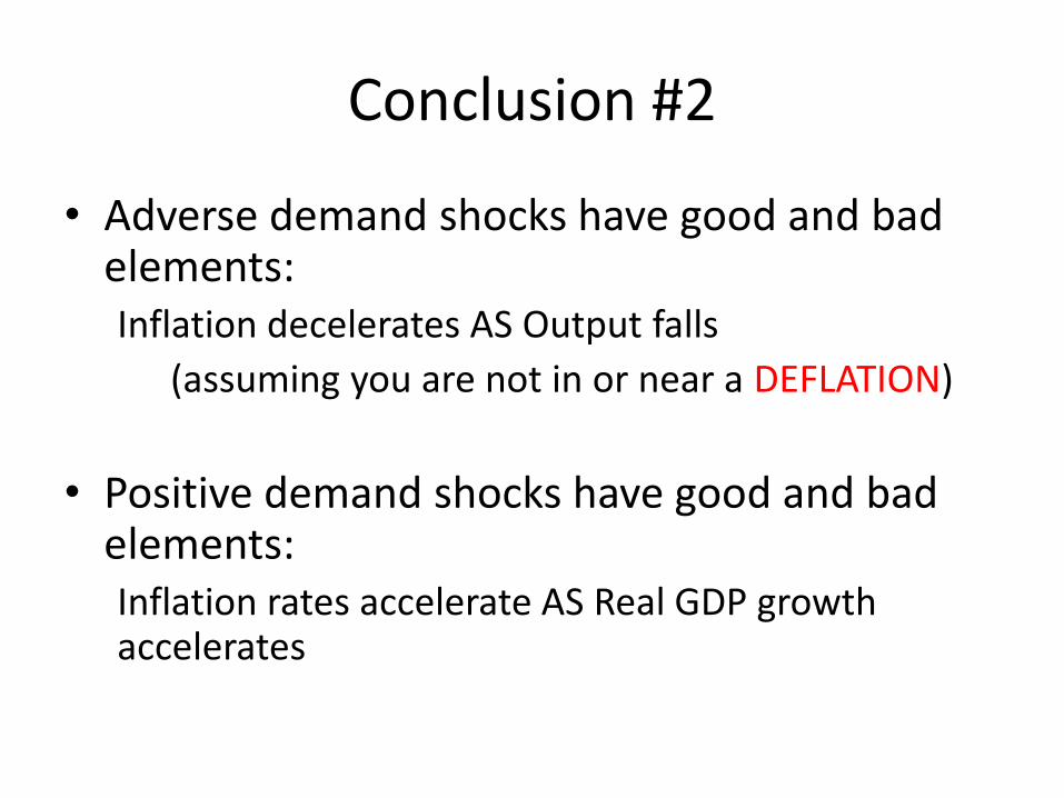
Conclusion #2

• Adverse demand shocks have good and bad elements: Inflation decelerates AS Output falls

(assuming you are not in or near a DEFLATION)

• Positive demand shocks have good and bad elements:Inflation rates accelerate AS Real GDP growth accelerates

SOME ADVERTISING FOR CFE

• The Financial Economics minor starts with basic footings in economics and builds a bridge to understanding the rich interaction between theory and practice in financial markets.

• The minor is open to all majors. Some required courses have prerequisites.

• Required courses:

• 180.101 Elements of Microeconomics

• 180.102 Elements of Macroeconomics

• 180.263 Corporate Finance

• 180.367 Investments & Portfolio Management

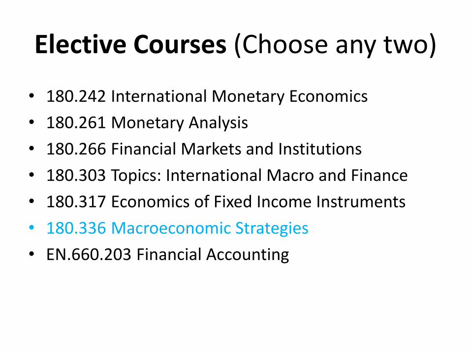
Elective Courses (Choose any two)

• 180.242 International Monetary Economics

• 180.261 Monetary Analysis

• 180.266 Financial Markets and Institutions

• 180.303 Topics: International Macro and Finance

• 180.317 Economics of Fixed Income Instruments

• 180.336 Macroeconomic Strategies

• EN.660.203 Financial Accounting