ECEN 615Methods of Electric Power

Systems Analysis

Lecture 16: State Estimation, EMS

Prof. Tom Overbye

Dept. of Electrical and Computer Engineering

Texas A&M University

overbye@tamu.edu

Announcements

• Read Chapter 9

• Homework 4 is due today

• In problem 5 the LODF is a vector

• In problem 6 find the OTDF on the line between buses 1

and 2

1

Electric Grid Measurements

• The two major types of measurements are voltages and

currents

– The challenge for both types are doing these measurements at

the high electric grid voltage levels

• Potential transformers (PTs) are used to measure

voltage, using a transformer sometimes

with a set

of series

capacitors

to drop the

voltage

2Image source: www.electrical4u.com/instrument-transformers/

Electric Grid Measurements

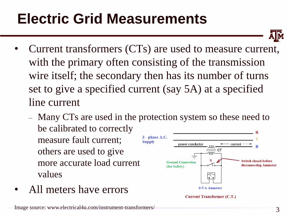
• Current transformers (CTs) are used to measure current,

with the primary often consisting of the transmission

wire itself; the secondary then has its number of turns

set to give a specified current (say 5A) at a specified

line current

– Many CTs are used in the protection system so these need to

be calibrated to correctly

measure fault current;

others are used to give

more accurate load current

values

• All meters have errors

3Image source: www.electrical4u.com/instrument-transformers/

Phasor Measurement Units (PMUs)

• All AC signals have a magnitude and phase. It is very

easy to measure the phase angle differences between

local signals (e.g., at an electrical substation)

– These differences are used to calculate power values

• However, it had been challenging to measure phase

angle differences between signals at different locations

– This requires access to a

precise time source

– At 60 Hz one cycle takes

16.67 ms, which means

one degree takes

46 ms.

4

Phasor Measurement Units (PMUs)

• Widespread access to precise time became available in

the 1980’s when civilian use of the GPS was allowed

• PMUs use the GPS signals to determine the phase

angles of voltages and currents (relative to some

global reference)

– The inputs to PMUs come from the CTs and PTs

• PMUs sample the system at rates on the order of 30

times per second

• PMU values are being used in SE algorithms

5

SE Example: Two Bus Case

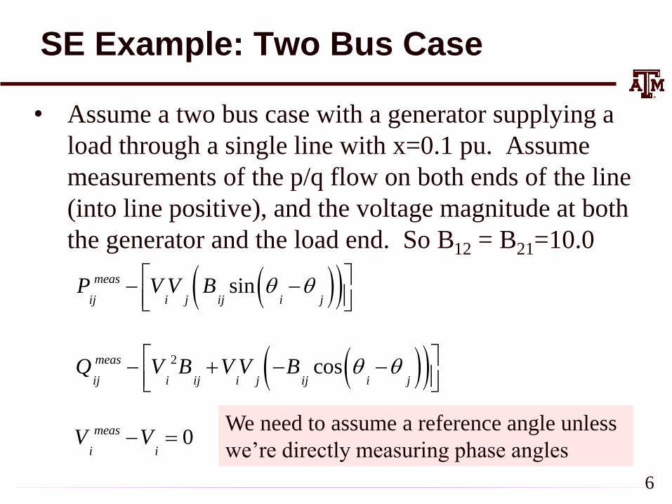
• Assume a two bus case with a generator supplying a

load through a single line with x=0.1 pu. Assume

measurements of the p/q flow on both ends of the line

(into line positive), and the voltage magnitude at both

the generator and the load end. So B12 = B21=10.0

( )( )

( )( )2

sin

cos

0

meas

ij i j ij i j

meas

ij i ij i j ij i j

meas

i i

P V V B

Q V B V V B

V V

− −

− + − −

− =We need to assume a reference angle unless

we’re directly measuring phase angles

6

Example: Two Bus Case

• Let .

.

., .

.

.

12

12

1

21meas 0

2 i

21

2

1

2

P 2 02

Q 1 5V 1

P 1 98x 0 0 01

Q 1V 1

V 1 01

V 0 87

−

= = = = = −

Z

sin( ) cos( ) sin( )

cos( ) sin( ) cos( )

sin( ) cos( ) sin( )( )

cos( ) sin( ) cos( )

2 2 1 2 2 1 2

1 2 2 1 2 2 1 2

2 2 1 2 2 1 2

2 2 1 2 2 2 1 2

V 10 V V 10 V 10

20V V 10 V V 10 V 10

V 10 V V 10 V 10H

V 10 V V 10 20V V 10

1 0 0

0 0 1

− − − −

− − − − − −

= − −

x

We assume an

angle reference

of 1=0

7

Example: Two Bus Case

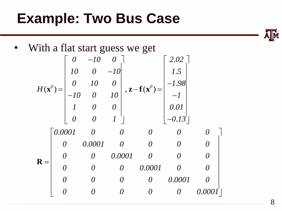
• With a flat start guess we get.

.

.( ) , ( )

.

.

.

.

.

.

.

.

0 0

0 10 0 2 02

10 0 10 1 5

0 10 0 1 98H

10 0 10 1

1 0 0 0 01

0 0 1 0 13

0 0001 0 0 0 0 0

0 0 0001 0 0 0 0

0 0 0 0001 0 0 0

0 0 0 0 0001 0 0

0 0 0 0 0 0001 0

0 0 0 0 0 0 0001

−

− −

= − = − −

−

=

x z f x

R

8

Example: Two Bus Case

1 6

11 0 1 1

2.01 0 2

1 0 2 0

2 0 2.01

2.02

1.51.003

1.980.2

10.8775

0.01

0.13

T

T T

e−

−− −

−

= −

− = + = − − −

H R H

x x H R H H R

9

Assumed SE Measurement Accuracy

• The assumed measurement standard deviations can

have a significant impact on the resultant solution, or

even whether the SE converges

• The assumption is a Gaussian (normal) distribution of

the error with no bias

10

SE Observability

• In order to estimate all n states we need at least n

measurements. However, where the measurements are

located is also important, a topic known as observability

– In order for a power system to be fully observable usually we

need to have a measurement available no more than one bus

away

– At buses we need to have at least measurements on all the

injections into the bus except one (including loads and gens)

– Loads are usually flows on feeders, or the flow into a

transmission to distribution transformer

– Generators are usually just injections from the GSU

11

Pseudo Measurements

• Pseudo measurements are used at buses in which there

is no load or generation; that is, the net injection into

the bus is know with high accuracy to be zero

– In order to enforce the net power balance at a bus we need to

include an explicit net injection measurement

• To increase observability sometimes estimated values

are used for loads, shunts and generator outputs

– These “measurements” are represented as having a higher

much standard deviation

12

SE Observability Example

13

SE Bad Data Detection

• The quality of the measurements available to an SE

can vary widely, and sometimes the SE model itself is

wrong. Causes include

– Modeling Errors: perhaps the assumed system topology is

incorrect, or the assumed parameters for a transmission line

or transformer could be wrong

– Data Errors: measurements may be incorrect because of in

correct data specifications, like the CT ratios or even flipped

positive and negative directions

– Transducer Errors: the transductors may be failing or may

have bias errors

– Sampling Errors: SCADA does not read all values

simultaneously and power systems are dynamic14

SE Bad Data Detection

• The challenge for SE is to determine when there is

likely a bad measurement (or multiple ones), and then

to determine the particular bad measurements

• J(x) is random number, with a probability density

function (PDF) known as a chi-squared distribution,

2(K), where K is the degrees of freedom, K=m-n

• It can be shown the expected mean for J(x) is K, with a

standard deviation of

– Values of J(x) outside of several standard deviations indicate

possible bad measurements, with the measurement residuals

used to track down the likely bad measurements

• SE can be re-run without the bad measurements 15

2K

QR Factorization

• Used in SE since it handles ill-conditioned m by n

matrices (with m >= n)

• Can be used with sparse matrices

• We will first split the R-1 matrix

• QR factorization represents the m by n H' matrix as

with Q an m by m orthonormal matrix and U an upper

triangular matrix (most books use Q R but we use U to

avoid confusion with the previous R)

1 11 2 2T T T− −− = =H R H H R R H H H

=H QU

16

Orthonormal Matrices

• The term orthogonal is used with vectors to indicate

their dot product is zero (i.e., they are perpendicular to

each other)

• Orthonormal is used to indicate they are orthogonal

and each has unit length (magnitude of 1)

• The definition of an orthogonal matrix is QTQ = I

– This implies its inverse always exists

• Its determinant is 1

• They can be used for transformations such as an

angular rotation

17

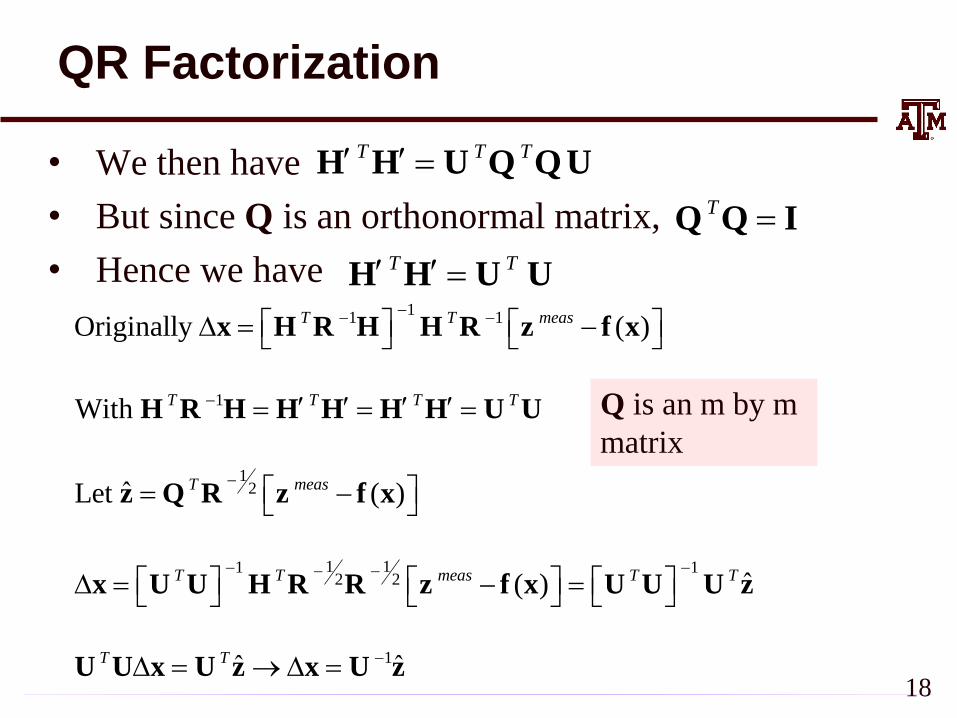
QR Factorization

• We then have

• But since Q is an orthonormal matrix,

• Hence we have

T T T =H H U Q QU

T =Q Q I

T T =H H U U1

1 1

1

12

1 11 12 2

1

Originally ( )

With

ˆLet ( )

ˆ( )

ˆ ˆ

T T meas

T T T T

T meas

T T meas T T

T T

−− −

−

−

− −− −

−

= −

= = =

= −

= − =

= → =

x H R H H R z f x

H R H H H H H U U

z Q R z f x

x U U H R R z f x U U U z

U U x U z x U z18

Q is an m by m

matrix

QR Factorization

• Next we’ll briefly discuss the QR factorization

algorithm

• When factored the U matrix (i.e., what most call the R

matrix ) will be an m by n upper triangular matrix

• Several methods are available including the

Householder method and the Givens method

• Givens is preferred when dealing with sparse matrices

• A good reference is Gene H. Golub and Charles F. Van

Loan, “Matrix Computations,” second edition, Johns

Hopkins University Press, 1989.

19

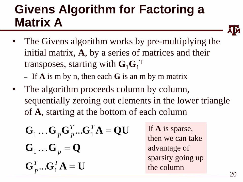
Givens Algorithm for Factoring a Matrix A

• The Givens algorithm works by pre-multiplying the

initial matrix, A, by a series of matrices and their

transposes, starting with G1G1T

– If A is m by n, then each G is an m by m matrix

• The algorithm proceeds column by column,

sequentially zeroing out elements in the lower triangle

of A, starting at the bottom of each column

1 1

1

1

...

...

T T

p p

p

T T

p

=

=

=

G G G G A QU

G G Q

G G A U

If A is sparse,

then we can take

advantage of

sparsity going up

the column20

Givens Algorithm

• To zero out element A[i,j], with i > j we first solve

with a=A[k,j], b= A[i,j]

• A numerically safe algorithm is

0

c s a r

s c b

− =

2

2

If b=0 then c=1, s=0 // i.e, no rotation is needed

Else If / ; 1/ 1 ;

Else

b > a th|

/ ; 1/ 1 ;

n| e a b s c s

b a c s c

= − = + =

= − = + =

To zero out an element

we need a non-zero

pivot element in column j;

assume this row as k. 2 2r a b= +

21

Givens G Matrix

• The orthogonal G(i,k,) matrix is then

• Premultiplication by G(i,k,)T is a rotation by

radians in the (i,k) coordinate plane

1 0 0 0

0 0

( ,k, )

0 0

0 0 0 1

c s

i

s c

= −

G

As noted, to zero out an

element we need a non-zero

pivot element in column j;

assume this row as k. Row

k here is the first non-zero

above row i.

22

Small Givens Example

• Let

• First we zero out A[4,1], a=1, b=2 giving s= 0.8944,

c=-0.4472

4 2

1 0

0 5

2 1

=

A

1 1

1 0 0 0 4 2

0 0.4472 0 0.8944 2.236 0.8944

0 0 1 0 0 5

0 0.8944 0 0.4472 0 0.4472

T

− − − = =

− − −

G G A

23

First start in column j=1; we will

zero out A[4,1] with i=4, k=2

Small Givens Example

• Next zero out A[2,1] with a=4, b=-2.236, giving

c= -0.8729, s=0.4880

• Next zero out A[4,2] with a=5, b=-0.447, c=0.996,

s=0.089

2 2 1

0.873 0.488 0 0 4.58 2.18

0.488 0.873 0 0 0 0.195

0 0 1 0 0 5

0 0 0 1 0 0.447

T T

−

= =

−

G G G A

24

3 3 2 1

1 0 0 0 4.58 2.18

0 1 0 0 0 0.195

0 0 0.996 0.089 0 5.020

0 0 0.089 0.996 0 0

T T T

= =

−

G G G G A

k=1 with A[k,j]=4

j=2, k=3 with A[k,j]=5

Small Givens Example

• Next zero out A[3,2] with a=0.195, b=5.02, c=-0.039,

s=0.999

• Also we have

4 4 3 2 1

1 0 0 0 4.58 2.18

0 0.039 0.999 0 0 5.023

0 0.999 0.039 0 0 0

0 0 0 1 0 0

T T T T

− − = = = − −

G G G G G A U

1 2 3 4

0.872 0.019 0.487 0

0.218 0.094 0.387 0.891

0 0.995 0.039 0.089

0.436 0.009 0.782 0.445

−

− = = − −

− − −

Q G G G G

25

j=2, k=2 with A[k,j]=0.195

Start of Givens for SE Example

• Starting with the H matrix we get

• To zero out H'[5,1]=1 we have

b=100, a=-1000, giving

c=0.995, s=0.0995

12

0 10 0

10 0 10

0 10 0100

10 0 10

1 0 0

0 0 1

−

−

−

= = −

H R H

1

1 0 0 0 0 0

0 1 0 0 0 0

0 0 1 0 0 0

0 0 0 0.995 0.0995 0

0 0 0 0.0995 0.995 0

0 0 0 0 0 1

= −

G

26

Here the column (j) is 1, while

i is 5 and k is 4.

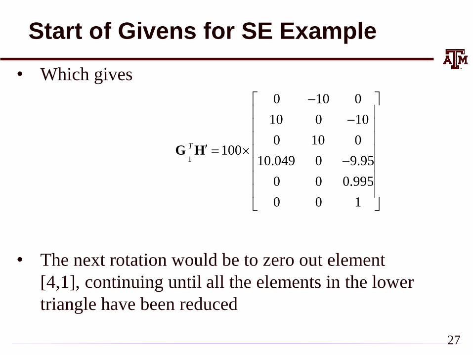
Start of Givens for SE Example

• Which gives

• The next rotation would be to zero out element

[4,1], continuing until all the elements in the lower

triangle have been reduced

1

0 10 0

10 0 10

0 10 0100

10.049 0 9.95

0 0 0.995

0 0 1

T

−

−

= −

G H

27

Givens Comments

• For a full matrix, Givens is O(mn2) since each element

in the lower triangle needs to be zeroed O(nm), and

each operation is O(n)

• Computation can be drastically reduced for a sparse

matrix since we only need to zero out the elements that

are initially non-zero, and any that become non-zero

(i.e., the fills)

– Also, for each multiply we only need to deal with the

nonzeros in the impacted row

• Givens rotation is commonly used to solve the SE

28

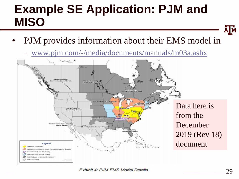
Example SE Application: PJM and MISO

• PJM provides information about their EMS model in

– www.pjm.com/-/media/documents/manuals/m03a.ashx

Data here is

from the

December

2019 (Rev 18)

document

29

Example SE Application: PJM and MISO

• PJM measurements are required for 69 kV and up

• PJM SE is triggered to execute every minute

• PJM SE solves well over 98% of the time

• Below reference provides info on MISO SE from

March 2015

– 54,433 buses

– 54,415 network branches

– 6332 generating units

– 228,673 circuit breakers

– 289,491 mapped points

https://www.naspi.org/sites/default/files/2017-05/3a%20MISO-NASPIWokshop-

Synchrophasor%20Data%20and%20State%20Estimation.pdf30

Energy Management Systems (EMSs)

• EMSs are now used to control most large scale

electric grids

• EMSs developed in the 1970’s and 1980’s out of

SCADA systems

– An EMS usually includes a SCADA system; sometimes

called a SCADA/EMS

• Having a SE is almost the definition of an EMS. The

SE then feeds data to the more advanced functions

• EMSs have evolved as the industry as evolved as the

industry has evolved, with functionality customized

for the application (e.g., a reliability coordinator or a

vertically integrated utility) 31

NERC Reliability Coordinators

Source: www.nerc.com/pa/rrm/TLR/Pages/Reliability-Coordinators.aspx32

EEI Member Companies

33

Electric Coops

34

Texas Electric Coops

35