EECS 142 Lecture 17: BJT/FET Mixers/Mixer Noise Prof. Ali M. Niknejad University of California, Berkeley Copyright c 2005 by Ali M. Niknejad A. M. Niknejad University of California, Berkeley EECS 142 Lecture 17 p. 1/35
A. M. Niknejad University of California, Berkeley EECS 142 Lecture 17 p. 1/35 – p. 1/35
A BJT Mixer
C∞
L1
C1
L2
C2
L3
C∞
C3
LO
RF
IF
The transformer is used to sum the LO and RF signalsat the input. The winding inductance is used to formresonant tanks at the LO and RF frequencies.
The output tank is tuned to the IF frequency.
Large capacitors are used to form AC grounds.
A. M. Niknejad University of California, Berkeley EECS 142 Lecture 17 p. 2/35 – p. 2/35
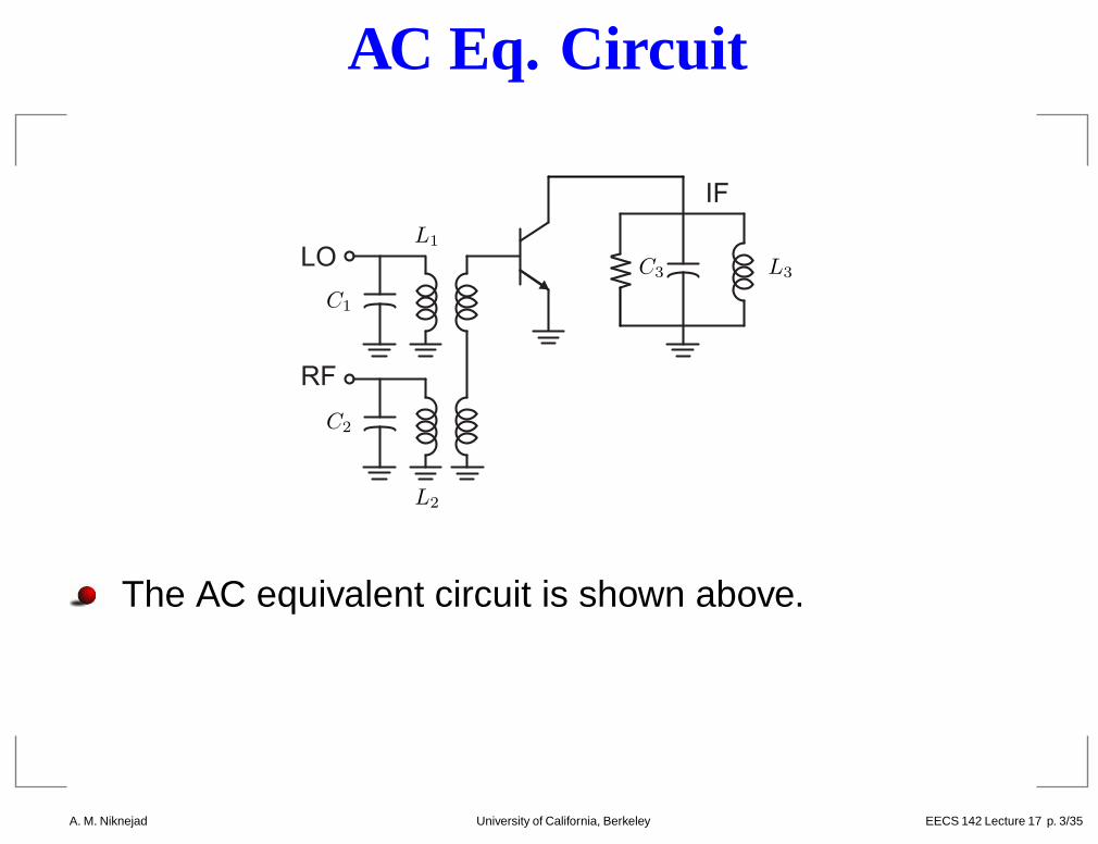
AC Eq. Circuit
L1
C1
L2
C2
L3C3LO
RF
IF
The AC equivalent circuit is shown above.
A. M. Niknejad University of California, Berkeley EECS 142 Lecture 17 p. 3/35 – p. 3/35
BJT Mixer Analysis
When we apply the LO alone, the collector current ofthe mixer is given by
IC = IQ
(
1 +2I1(b)
I0(b)cos ωt +
2I2(b)
I0(b)cos 2ωt + · · ·
)
We can therefore define a time-varying gm(t) by
gm(t) =IC(t)
Vt=
qIC(t)
kT
The output current when the RF is also applied istherefore given by iC(t) = gm(t)vs
iC =qIQ
kT
(
1 +2I1(b)
I0(b)cos ωt +
2I2(b)
I0(b)cos 2ωt + · · ·
)
×V̂s cos ωst
A. M. Niknejad University of California, Berkeley EECS 142 Lecture 17 p. 4/35 – p. 4/35
BJT Mixer Analysis (cont)The output at the IF is therefore given by
iC |ωIF= V̂s
qIQ
kT︸︷︷︸
gmQ
I1(b)
I0(b)cos(ω0 − ωs
︸ ︷︷ ︸
ωIF
)t
The conversion gain is given by
gconv = gmQI1(b)
I0(b)
2 4 6 8 10
0.2
0.4
0.6
0.8
1
gconv
gmQ
b =V̂i
VA. M. Niknejad University of California, Berkeley EECS 142 Lecture 17 p. 5/35 – p. 5/35
LO Signal Drive
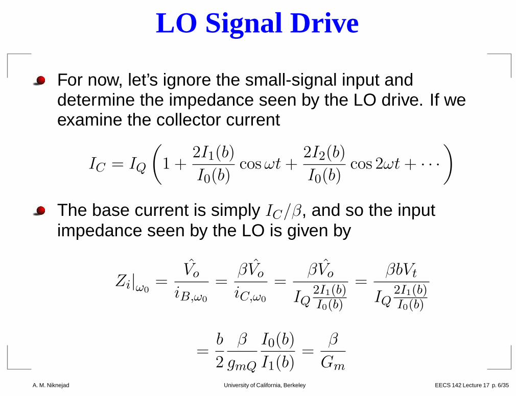
For now, let’s ignore the small-signal input anddetermine the impedance seen by the LO drive. If weexamine the collector current
IC = IQ
(
1 +2I1(b)
I0(b)cos ωt +
2I2(b)
I0(b)cos 2ωt + · · ·
)
The base current is simply IC/β, and so the inputimpedance seen by the LO is given by
Zi|ω0=
V̂o
iB,ω0
=βV̂o
iC,ω0
=βV̂o
IQ2I1(b)I0(b)
=βbVt
IQ2I1(b)I0(b)
=b
2
β
gmQ
I0(b)
I1(b)=
β
Gm
A. M. Niknejad University of California, Berkeley EECS 142 Lecture 17 p. 6/35 – p. 6/35
RF Signal Drive
The impedance seen by the RF singal source is alsothe base current at the ωs components. Typically, wehave a high-Q circuit at the input that resonates at RF.
iB(t) =iC(t)
β
=1
β
qIQ
kT
(
V̂s cos ωst +2I1(b)
I0(b)cos(ω0 ± ωs)t + · · ·
)
The input impedance is thus the same as an amplifier
Rin =V̂s
|component in iB at ωs|= β
kT
qIQ=
β
gmQ
A. M. Niknejad University of California, Berkeley EECS 142 Lecture 17 p. 7/35 – p. 7/35
Mixer Analysis: General Approach
If we go back to our original equations, our majorassumption was that the mixer is a linear time-varyingfunction relative to the RF input. Let’s see how thatcomes about
IC = ISevBE/Vt
wherevBE = vin + vo + VA
or
IC = ISeVA/Vt × eb cos ω0t × eV̂sVt
cos ωst
If we assume that the RF signal is weak, then we canapproximate ex ≈ 1 + x
A. M. Niknejad University of California, Berkeley EECS 142 Lecture 17 p. 8/35 – p. 8/35
General Approach (cont)
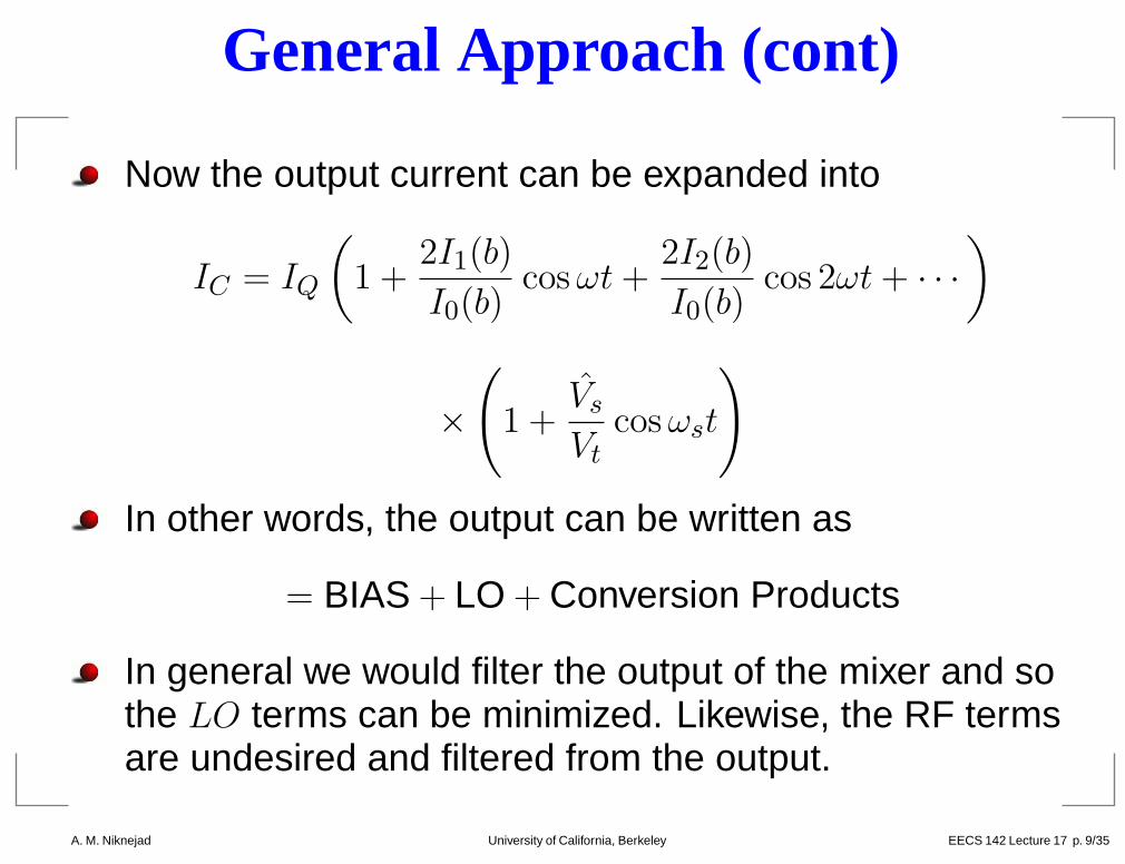
Now the output current can be expanded into
IC = IQ
(
1 +2I1(b)
I0(b)cos ωt +
2I2(b)
I0(b)cos 2ωt + · · ·
)
×
(
1 +V̂s
Vtcos ωst
)
In other words, the output can be written as
= BIAS + LO + Conversion Products
In general we would filter the output of the mixer and sothe LO terms can be minimized. Likewise, the RF termsare undesired and filtered from the output.
A. M. Niknejad University of California, Berkeley EECS 142 Lecture 17 p. 9/35 – p. 9/35
Distortion in Mixers
Using the same formulation, we can now insert a signalwith two tones
vin = V̂s1 cos ωs1t + V̂s2 cos ωs2
IC = ISeVA/Vt × eb cos ω0t × eˆVs1
Vtcos ωs1t+
ˆVs2Vt
cos ωs2t
The final term can be expanded into a Taylor series
IC = ISeVA/Vt × eb cos ω0t ×
(1 + Vs1 cos ωs1t + Vs2 cos ωs2t + ( )2 + ( )3 + · · ·
)
The square and cubic terms produce IM products asbefore, but now these products are frequency translatedto the IF frequency
A. M. Niknejad University of California, Berkeley EECS 142 Lecture 17 p. 10/35 – p
Another BJT Mixer
L3
C∞
C3LO
RF
IF
C0
CsLs
+v0x
The signal from the LO driver is capacitively coupled tothe BJT mixer
A. M. Niknejad University of California, Berkeley EECS 142 Lecture 17 p. 11/35 – p
LO Capacitive Divider
CsLs
+v0x
C0
+v0x
C0
C ′
s
Assume that ωLO > ωRF , or a high side injection
Note beyond resonance, the input impedance of thetank appears capacitive. Thus C ′
s is the effectivecapacitance of the tank. The equivalent circuit for theLO drive is therefore a capacitive divider
vo =Co
Co + C ′
svox
A. M. Niknejad University of California, Berkeley EECS 142 Lecture 17 p. 12/35 – p
Harmonic Mixer
Second
Harmonic
Mixer
LO
RF IF
We can use a harmonic of the LO to build a mixer.
Example, let LO = 500MHz, RF = 900MHz, andIF = 100MHz.
Note that IF = 2LO − RF = 1000 − 900 = 100
A. M. Niknejad University of California, Berkeley EECS 142 Lecture 17 p. 13/35 – p
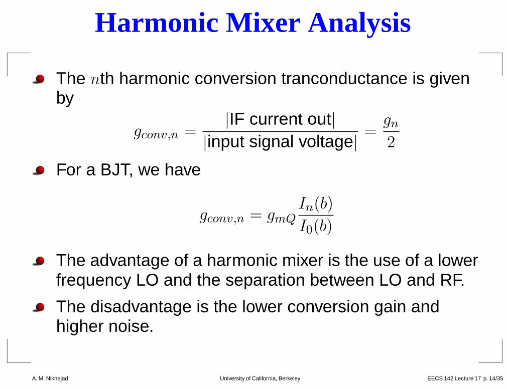
Harmonic Mixer Analysis
The nth harmonic conversion tranconductance is givenby
gconv,n =|IF current out|
|input signal voltage|=
gn
2
For a BJT, we have
gconv,n = gmQIn(b)
I0(b)
The advantage of a harmonic mixer is the use of a lowerfrequency LO and the separation between LO and RF.
The disadvantage is the lower conversion gain andhigher noise.
A. M. Niknejad University of California, Berkeley EECS 142 Lecture 17 p. 14/35 – p
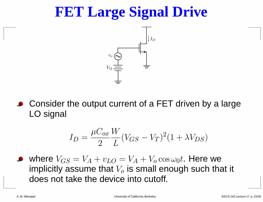
FET Large Signal Drive
vo
VQ
ID
Consider the output current of a FET driven by a largeLO signal
ID =µCox
2
W
L(VGS − VT )2(1 + λVDS)
where VGS = VA + vLO = VA + Vo cos ω0t. Here weimplicitly assume that Vo is small enough such that itdoes not take the device into cutoff.
A. M. Niknejad University of California, Berkeley EECS 142 Lecture 17 p. 15/35 – p
FET Large Signal Drive (cont)
0.5 1 1.5 2 2.5 3
That means that VA + V0 cos ω0t > VT , or VA − V0 > VT ,or equivalently V0 < VA − VT . Under such a case weexpand the current
ID ∝((VA − VT )2 + V0 cos2 ω0t + 2(VA − VT )V0 cos ω0t
)
A. M. Niknejad University of California, Berkeley EECS 142 Lecture 17 p. 16/35 – p
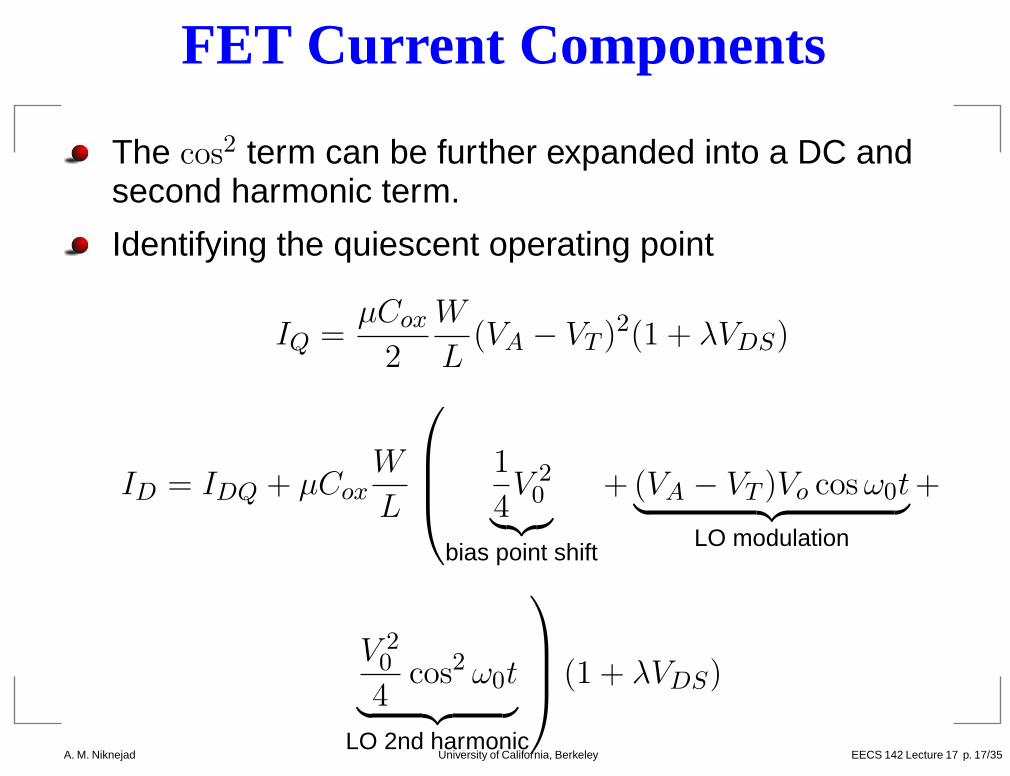
FET Current Components
The cos2 term can be further expanded into a DC andsecond harmonic term.
Identifying the quiescent operating point
IQ =µCox
2
W
L(VA − VT )2(1 + λVDS)
ID = IDQ + µCoxW
L
1
4V 2
0︸︷︷︸
bias point shift
+ (VA − VT )Vo cos ω0t︸ ︷︷ ︸
LO modulation
+
V 20
4cos2 ω0t
︸ ︷︷ ︸
LO 2nd harmonic
(1 + λVDS)
A. M. Niknejad University of California, Berkeley EECS 142 Lecture 17 p. 17/35 – p
FET Time-Varying Transconductance
The transconductance of a FET is given by (assumingstrong inversion operation)
g(t) =∂ID
∂VGS= µCox
W
L(VGS − VT )(1 + λVDS)
VGS(t) = VA + V0 cos ω0t
g(t) = µCoxW
L(VA − VT + V0 cos ω0t)(1 + λVDS)
g(t) = gmQ
(
1 +V0
VA − VTcos ω0t
)
(1 + λVDS)
This is an almost ideal mixer in that there is noharmonic components in the transconductance.
A. M. Niknejad University of California, Berkeley EECS 142 Lecture 17 p. 18/35 – p
MOS Mixer
vs
VQ
vo
IF Filter
We see that we can builda mixer by simply injectingan LO + RF signal at thegate of the FET (ignore out-put resistance)
i0 = g(t)vs = gmQ
(
1 +V0
VA − VTcos ω0t
)
Vs cos ωst
i0|IF =gmQ
2
V0
VA − VTcos(ω0 ± ωs)tVs
gc =i0|IF
Vs=
gmQ
2
V0
VA − VT
A. M. Niknejad University of California, Berkeley EECS 142 Lecture 17 p. 19/35 – p
MOS Mixer Summary
But gmQ = µCoxWL (VA − VT )
gc =µCox
2
W
LV0
which means that gc is independent of bias VA. Thegain is controlled by the LO amplitude V0 and by thedevice aspect ratio.
Keep in mind, though, that the transistor must remain inforward active region in the entire cycle for the aboveassumptions to hold.
In practice, a real FET is not square law and the aboveanalysis should be verified with extensive simulation.Sub-threshold conduction and output conductancecomplicate the picture.
A. M. Niknejad University of California, Berkeley EECS 142 Lecture 17 p. 20/35 – p
“Dual Gate” Mixer
+vs
M1
M2
VA
+vo
VA
io
G1
G2D2
S1
shared junction
(no contact)
The “dual gate” mixer, or more commonly a cascodeamplifier, can be turned into a mixer by applying the LOat the gate of M2 and the RF signal at the gate of M1.Using two transistors in place of one transistor results inarea savings since the signals do not need to becombined with a transformer or capacitively .
A. M. Niknejad University of California, Berkeley EECS 142 Lecture 17 p. 21/35 – p
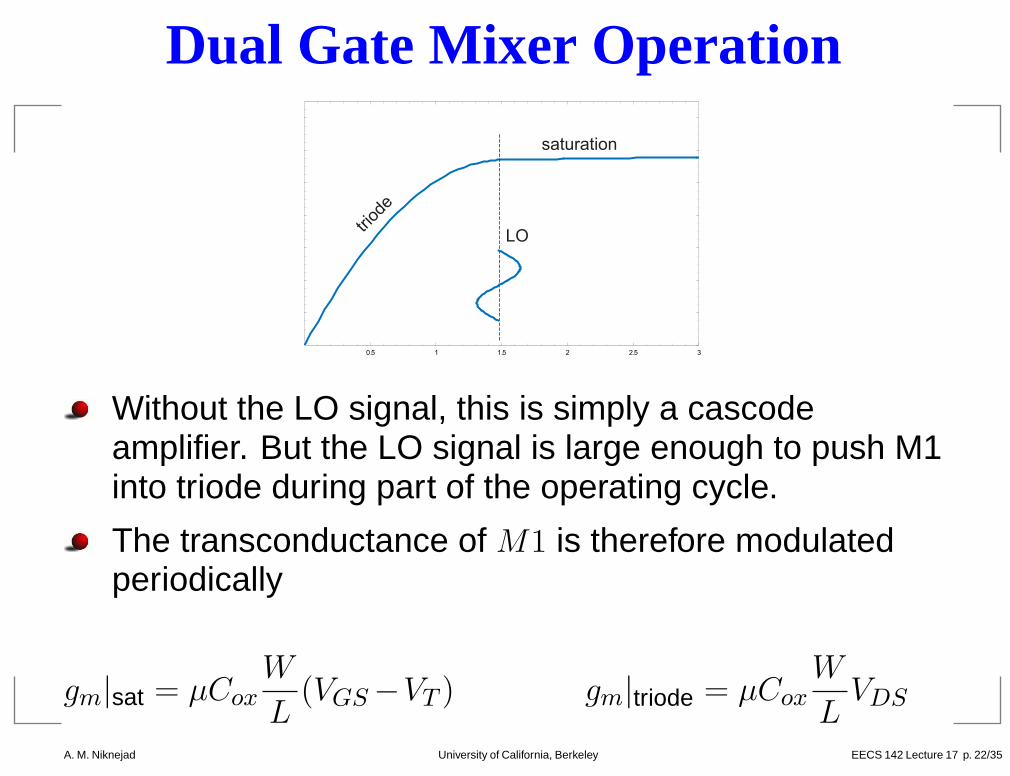
Dual Gate Mixer Operation
0.5 1 1.5 2 2.5 3
triod
e
saturation
LO
Without the LO signal, this is simply a cascodeamplifier. But the LO signal is large enough to push M1into triode during part of the operating cycle.
The transconductance of M1 is therefore modulatedperiodically
gm|sat = µCoxW
L(VGS −VT ) gm|triode = µCox
W
LVDS
A. M. Niknejad University of California, Berkeley EECS 142 Lecture 17 p. 22/35 – p
Dual Gate Waveforms
Active Region
Triode Region
gm,max
gm(t)
vLO,1
vLO,2
VGS2 is roughly constant since M1 acts like a currentsource.
VD1 = vLO − VGS2 = VA2 + V0 cos ω0t − VGS2
g(t) =
{
µCoxWL (VGS1 − VT ) VD1 > VGS − VT
µCox(VA2 − VGS2 − |V0 cos ω0t|) VD1 < VGS − VT
A. M. Niknejad University of California, Berkeley EECS 142 Lecture 17 p. 23/35 – p
Realistic Waveforms
A more sophisticated analysis would take sub-thresholdoperation into account and the resulting g(t) curvewould be smoother. A Fourier decomposition of thewaveform would yield the conversion gain coefficient asthe first harmonic amplitude.
A. M. Niknejad University of California, Berkeley EECS 142 Lecture 17 p. 24/35 – p
Mixer Analysis: Time Domain
A generic mixer operates with a periodic transferfunction h(t + T ) = h(t), where T = 1/ω0, or T is the LOperiod. We can thus expand h(t) into a Fourier series
y(t) = h(t)x(t) =∞∑
−∞
cnejω0ntx(t)
For a sinusoidal input, x(t) = A(t) cos ω1t, we have
y(t) =∞∑
−∞
cn
2A(t)
(
ej(ω1+ω0n)t + ej(−ω1+ω0n)t)
Since h(t) is a real function, the coefficients c−k = ck areeven. That means that we can pair positive andnegative frequency components.
A. M. Niknejad University of California, Berkeley EECS 142 Lecture 17 p. 25/35 – p
Unlike a perfect multiplier, we get an infinite number offrequency translations up and down by harmonics of ω0.
A. M. Niknejad University of California, Berkeley EECS 142 Lecture 17 p. 26/35 – p
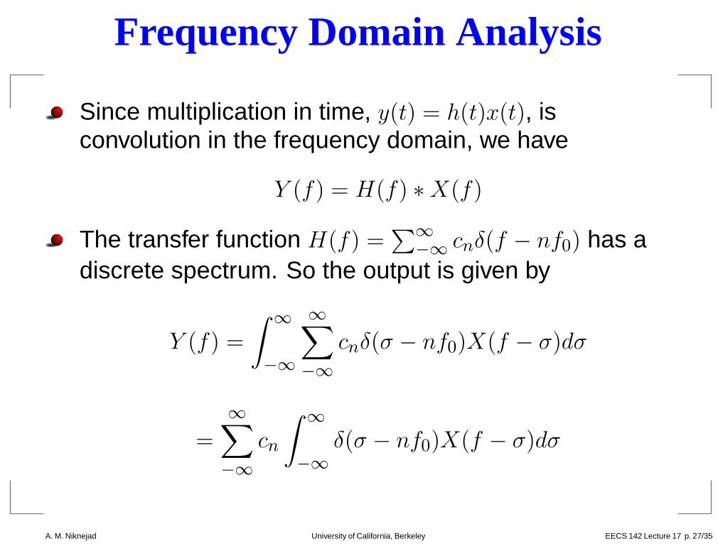
Frequency Domain Analysis
Since multiplication in time, y(t) = h(t)x(t), isconvolution in the frequency domain, we have
Y (f) = H(f) ∗ X(f)
The transfer function H(f) =∑
∞
−∞cnδ(f − nf0) has a
discrete spectrum. So the output is given by
Y (f) =
∫∞
−∞
∞∑
−∞
cnδ(σ − nf0)X(f − σ)dσ
=∞∑
−∞
cn
∫∞
−∞
δ(σ − nf0)X(f − σ)dσ
A. M. Niknejad University of California, Berkeley EECS 142 Lecture 17 p. 27/35 – p
Frequency Domain (cont)
noise folding from 3LO
noise folding from
2LO noise
folding fro
m -2LO
n
oise folding from -3LO
fo fsfif
−fo
−fs
−fif 2fo 3fo
−2fo
−3fo
By the frequency sifting property of the δ(f − σ)function, we have
Y (f) =∞∑
−∞
cnX(f − nf0)
Thus, the input spectrum is shifted by all harmonics ofthe LO up and down in frequency.
A. M. Niknejad University of California, Berkeley EECS 142 Lecture 17 p. 28/35 – p
Noise/Image Problem
Previously we examined the “image” problem. Anysignal energy a distance of IF from the LO getsdownconverted in a perfect multiplier. But now we seethat for a general mixer, any signal energy with an IF ofany harmonic of the LO will be downconverted !
These other images are easy to reject because they aredistant from the desired signal and a image reject filterwill be able to attenuate them significantly.
The noise power, though, in all image bands will foldonto the IF frequency. Note that the noise is generatedby the mixer source resistance itself and has a whitespectrum. Even though the noise of the antenna isfiltered, new noise is generated by the filter itself!
A. M. Niknejad University of California, Berkeley EECS 142 Lecture 17 p. 29/35 – p
Current Commutating Mixers
+LO −LO
VCC
Q2 Q3
Q1+RF
IF
RIF
+LO −LO
+RF
IF
A popular alternative mixer topology uses a differentialpair LO drive and an RF current injection at the tail. Inpractice, the tail current source is implemented as atransconductor.
The LO signal is large enough to completely steer theRF current either through Q1 or Q2.
A. M. Niknejad University of California, Berkeley EECS 142 Lecture 17 p. 30/35 – p
Current Commutating Mixer Model
+LO
−LO
VCC
Q1+RF
IF
RIF
If we model the circuit with ideal elements, we see thatthe current IC1 is either switched to the output or tosupply at the rate of the LO signal.
When the LO signal is positive, we have a cascodedumping its current into the supply. When the LO signalis negative, though, we have a cascode amplifier drivingthe output.
A. M. Niknejad University of California, Berkeley EECS 142 Lecture 17 p. 31/35 – p
Conversion Gain
tTLO
+1
0
s(t)
We can now see that the output current is given by aperiodic time varying transconductance
io = gm(t)vs = gmQs(t)vs
where s(t) is a square pulse waveform (ideally)switching between 1 and 0 at the rate of the LO signal.A Fourier decomposition yields
io = gmQvs
(
0.5 +2
πcos ω0t −
2
π
1
3cos 3ω0t + · · ·
)
A. M. Niknejad University of California, Berkeley EECS 142 Lecture 17 p. 32/35 – p
Conversion Gain (cont)
So the RF signal vs is amplified (feed-thru) by the DCterm and mixed by all the harmonics
ioVs
=gmQ
2
(1
2cos ωst +
2
πcos(ω0 ± ωs)t −
2
3πcos(3ω0 ± ωs)t + · · ·
)
The primary conversion gain is gc = 1πgmQ.
Since the role of Q1 (or M1) is to simply create an RFcurrent, it can be degenerated to improve the linearity ofthe mixer. Inductance degeneration can be employed toalso achieve an impedance match.
MOS version acts in a similar way but the conversiongain is lower (lower gm) and it requires a larger LO drive.
A. M. Niknejad University of California, Berkeley EECS 142 Lecture 17 p. 33/35 – p
Differential Output
+LO −LO
+RF
IF
This block is commonly known as the Gilbert Cell
If we take the output signal differentially, then the outputcurrent is given by
io = gm(t)vs = gmQs2(t)vs
A. M. Niknejad University of California, Berkeley EECS 142 Lecture 17 p. 34/35 – p
Differential Output Gain
t
TLO
+1
−1s2(t)
The pulse waveform s2(t) now switches between ±1,and thus has a zero DC value
s2(t) =4
πcos ω0t −
1
3
4
πcos 3ω0t + · · ·
The lack of the DC term means that there is ideally noRF feedthrough to the IF port. The conversion gain isdoubled since we take a differential output gc/gmQ = 2
π
A. M. Niknejad University of California, Berkeley EECS 142 Lecture 17 p. 35/35 – p