11/13/18 1 ECE 241 – Advanced Programming I Fall 2018 Mike Zink Lecture 17 Divide and Conquer – Fast Fourier Transform (FFT) Introduction • In several cases, it is desirable to evaluate a signal in the frequency domain as it gives a more insightful information about it. • A few use cases of FFT: – audio processing to clear noise – image processing to smooth images – OFDM (used in cellular communication) – speech recognition – audio fingerprinting (apps like Shazam and SoundHound)
Transcript
11/13/18
1
ECE241–AdvancedProgrammingIFall2018MikeZink
Lecture17DivideandConquer–
FastFourierTransform(FFT)
Introduction• In several cases, it is desirable to evaluate a signal in the
frequency domain as it gives a more insightful information about it.
• A few use cases of FFT:– audio processing to clear noise– image processing to smooth images– OFDM (used in cellular communication)– speech recognition– audio fingerprinting (apps like Shazam and SoundHound)
11/13/18
2
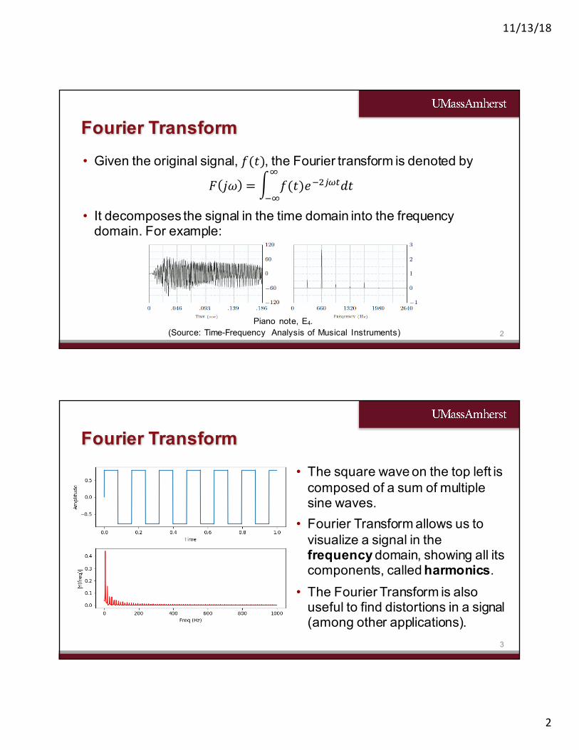
• Given the original signal, 𝑓(𝑡), the Fourier transform is denoted by
𝐹 𝑗𝜔 = ) 𝑓(𝑡)𝑒+,-./𝑑𝑡1
+1
• It decomposes the signal in the time domain into the frequency domain. For example:
2
Fourier Transform
Piano note, E4. (Source: Time-Frequency Analysis of Musical Instruments)
• The square wave on the top left is composed of a sum of multiple sine waves.
• Fourier Transform allows us to visualize a signal in the frequency domain, showing all its components, called harmonics.
• The Fourier Transform is also useful to find distortions in a signal (among other applications).
3
Fourier Transform
11/13/18
3
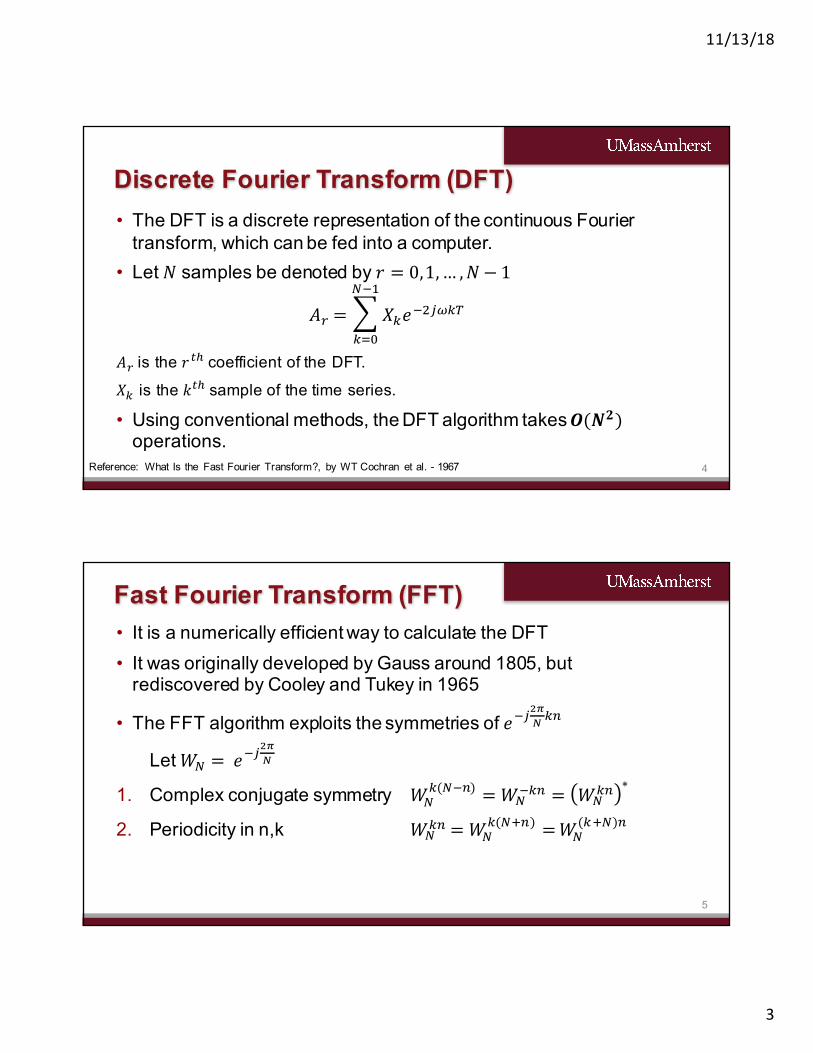
• The DFT is a discrete representation of the continuous Fourier transform, which can be fed into a computer.
• Let 𝑁 samples be denoted by 𝑟 = 0,1,… ,𝑁 − 1
𝐴: = ; 𝑋=𝑒+,-.=>?+@
=AB
𝐴: is the 𝑟/C coefficient of the DFT.
𝑋= is the 𝑘/C sample of the time series.
• Using conventional methods, the DFT algorithm takes 𝑶(𝑵𝟐)operations.
4
Discrete Fourier Transform (DFT)
Reference: What Is the Fast Fourier Transform?, by WT Cochran et al. - 1967
• It is a numerically efficient way to calculate the DFT• It was originally developed by Gauss around 1805, but
rediscovered by Cooley and Tukey in 1965
• The FFT algorithm exploits the symmetries of 𝑒+-HIJ =K
Let 𝑊? =𝑒+-HIJ
1. Complex conjugate symmetry 𝑊?=(?+K) = 𝑊?
+=K = 𝑊?=K ∗
2. Periodicity in n,k 𝑊?=K = 𝑊?
=(?OK) =𝑊?(=O?)K
5
Fast Fourier Transform (FFT)
11/13/18
4
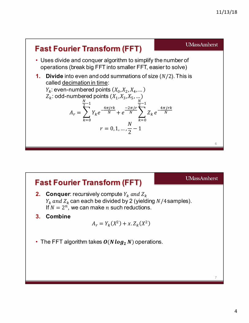
• Uses divide and conquer algorithm to simplify the number of operations (break big FFT into smaller FFT, easier to solve)
1. Divide into even and odd summations of size (𝑁/2). This is called decimation in time:𝑌=: even-numbered points 𝑋B,𝑋,, 𝑋S,…𝑍=: odd-numbered points (𝑋@,𝑋U,𝑋V,…)
𝐴: = ; 𝑌=𝑒+SW-:=?
?,+@
=AB
+ 𝑒+,W-:? ; 𝑍=
?,+@
=AB
𝑒+SW-:=?
𝑟 = 0,1,… ,𝑁2 − 1
6
Fast Fourier Transform (FFT)
2. Conquer: recursively compute𝑌=𝑎𝑛𝑑𝑍=𝑌=𝑎𝑛𝑑𝑍=can each be divided by 2 (yielding 𝑁/4samples). If 𝑁 = 2K, we can make 𝑛 such reductions.
3. Combine𝐴: = 𝑌= 𝑋, + 𝑥. 𝑍= 𝑋,
• The FFT algorithm takes 𝑶(𝑵𝒍𝒐𝒈𝟐 𝑵)operations.
7
Fast Fourier Transform (FFT)
11/13/18
5
8
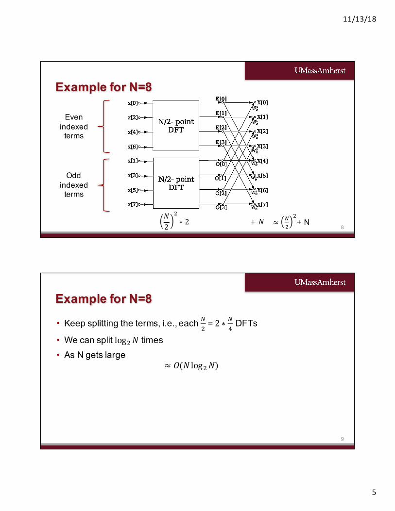
Example for N=8
Even indexed
terms
Odd indexed
terms
𝑁2
,∗ 2 +𝑁 ≈ ?
,
,+ N
• Keep splitting the terms, i.e., each ?,
= 2 ∗ ?S
DFTs
• We can split log,𝑁 times• As N gets large
≈ 𝑂(𝑁log,𝑁)
9
Example for N=8
11/13/18
6
10
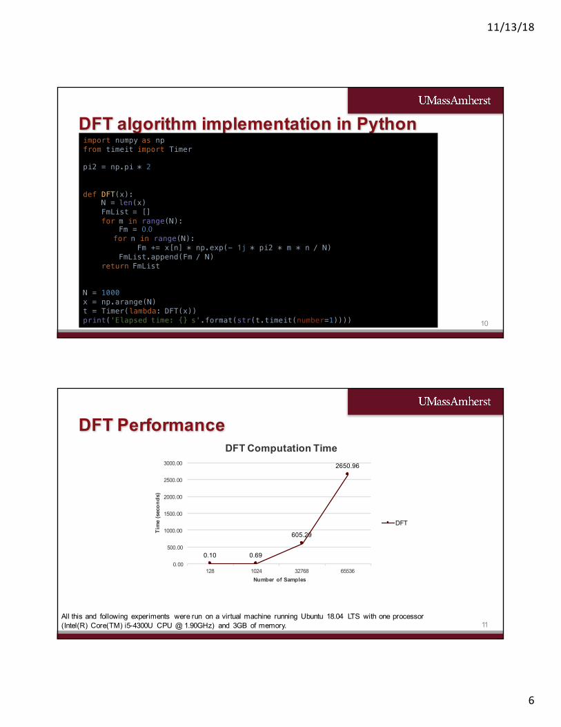
DFT algorithm implementation in Pythonimport numpy as npfrom timeit import Timer
pi2 = np.pi * 2
def DFT(x):N = len(x) FmList = [] for m in range(N):
Fm = 0.0 for n in range(N):
Fm += x[n] * np.exp(- 1j * pi2 * m * n / N) FmList.append(Fm / N)
All this and following experiments were run on a virtual machine running Ubuntu 18.04 LTS with one processor (Intel(R) Core(TM) i5-4300U CPU @ 1.90GHz) and 3GB of memory.
11/13/18
7
12
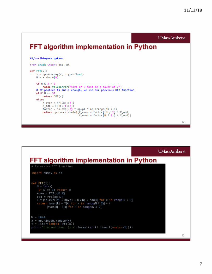
FFT algorithm implementation in Python
13
FFT algorithm implementation in Python# Recursive FFT function
import numpy as np
def FFT(x): N = len(x)
if N <= 1: return x even = FFT(x[0::2]) odd = FFT(x[1::2]) T = [np.exp(-2j * np.pi * k / N) * odd[k] for k in range(N // 2)] return [even[k] + T[k] for k in range(N // 2)] + \ [even[k] - T[k] for k in range(N // 2)] N = 1024x = np.random.random(N)t = Timer(lambda: FFT(x))print('Elapsed time: {} s'.format(str(t.timeit(number=1))))
11/13/18
8
14
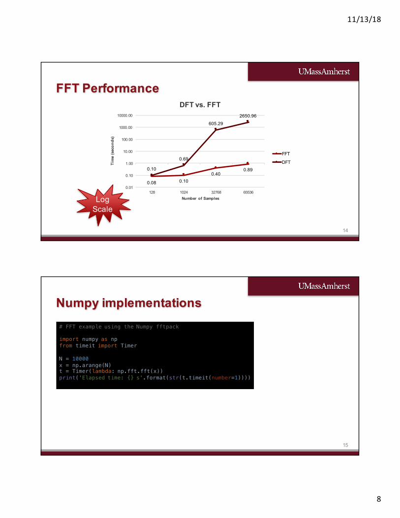
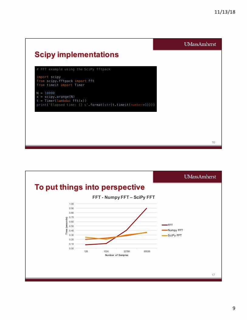
FFT Performance
0.08 0.100.40
0.890.10
0.69
605.292650.96
0.01
0.10
1.00
10.00
100.00
1000.00
10000.00
128 1024 32768 65536
Tim
e (s
econ
ds)
Number of Samples
DFT vs. FFT
FFT
DFT
Log Scale
15
Numpy implementations# FFT example using the Numpy fftpack
• Audio fingerprinting is a signature that summarizes an audio recording
• Also known as Content-Based audio Identification (CBID)• The best known application are apps like Shazam and
SoundHound, that link unlabeled audio recordings to a corresponding metadata (song name and artist, for instance)
18
Application – Audio Fingerprinting
Source: http://willdrevo.com/fingerprinting-and-audio-recognition-with-python/ for all following slides, unless otherwise stated
• Sampling: the standard sampling rate in digital music, such as HIFI, is 44,100 samples per second (from Nyquist theorem – 2 x 20 kHz)
• Quantization: the standard quantization uses 16 bits, or 65,536 levels
• PCM or Pulse Code Modulation: is the representation of the analog signal into zeros and ones
• This means that each second of music will have 44,100 samples per channel (one channel – Mono; two channels – Stereo)E.g.: 3 minutes of stereo song will have 15,876,000 samples
19
Background on Digital Audio
11/13/18
11
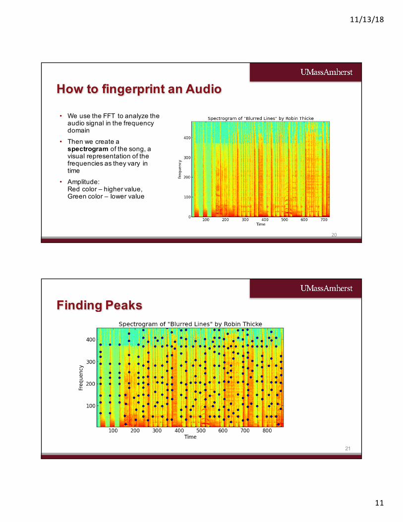
• We use the FFT to analyze the audio signal in the frequency domain
• Then we create a spectrogram of the song, a visual representation of the frequencies as they vary in time
• Amplitude:Red color – higher value, Green color – lower value
20
How to fingerprint an Audio
21
Finding Peaks
11/13/18
12
22
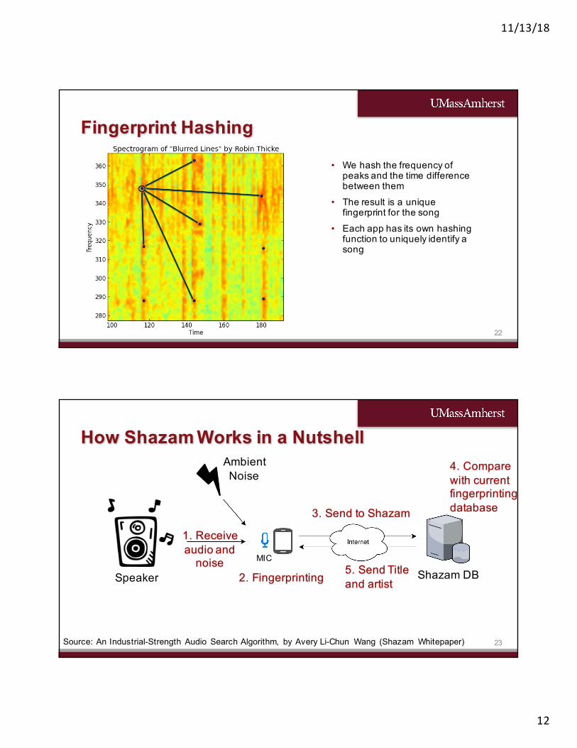
Fingerprint Hashing
• We hash the frequency of peaks and the time difference between them
• The result is a unique fingerprint for the song
• Each app has its own hashing function to uniquely identify a song
23
How Shazam Works in a Nutshell
Source: An Industrial-Strength Audio Search Algorithm, by Avery Li-Chun Wang (Shazam Whitepaper)