Lecture 18:Hypothesis testing IV:

Chi squareErnesto F. L. Amaral

October 31, 2017Advanced Methods of Social Research (SOCI 420)

Source: Healey, Joseph F. 2015. ”Statistics: A Tool for Social Research.” Stamford: Cengage Learning. 10th edition. Chapter 11 (pp. 276–306).

Chapter learning objectives• Identify and cite examples of situations in which the chi

square test is appropriate

• Explain the structure of a bivariate table and the concept of independence as applied to expected and observed frequencies in a bivariate table

• Explain the logic of hypothesis testing in terms of chi square

• Perform the chi square test using the five-step model and correctly interpret the results

• Explain the limitations of the chi square test and, especially, the difference between statistical significance and substantive significance (importance, magnitude)

2

The bivariate table• Bivariate tables display the scores of cases on

two different variables at the same time

3Source: Healey 2015, p.278.

Aspects of the table• Note the two dimensions: rows and columns • What is the independent variable?• What is the dependent variable? • Where are the row and column marginals?• Where is the total number of cases (N)?

4Source: Healey 2015, p.278.

Important information to report• Must have a title• Cells are intersections of columns and rows• Subtotals are called marginals• N is reported at the intersection of row and

column marginals

5

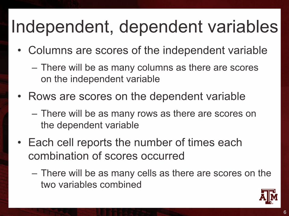
Independent, dependent variables• Columns are scores of the independent variable

– There will be as many columns as there are scores on the independent variable

• Rows are scores on the dependent variable– There will be as many rows as there are scores on

the dependent variable

• Each cell reports the number of times each combination of scores occurred– There will be as many cells as there are scores on the

two variables combined

6

Test for independence• Chi Square as a test of statistical significance is

a test for independence– Two variables are independent if the classification of

a case into a particular category of one variable has no effect on the probability that the case will fall into any particular category of the second variable

7Source: Healey 2015, p.279.

Cross tabulations• Chi Square is a test of significance based on

bivariate tables– Bivariate tables are also called cross tabulations,

crosstabs, contingency tables

• We are looking for significant differences between– The actual cell frequencies observed in a table (fo)– And those that would be expected by random chance

or if cell frequencies were independent (fe)

8

Computation of chi square

9

𝑓" =𝑅𝑜𝑤𝑚𝑎𝑟𝑔𝑖𝑛𝑎𝑙×𝐶𝑜𝑙𝑢𝑚𝑛𝑚𝑎𝑟𝑔𝑖𝑛𝑎𝑙

𝑁

𝜒4 𝑜𝑏𝑡𝑎𝑖𝑛𝑒𝑑 =9𝑓: − 𝑓" 4

𝑓"

�

�where fo = cell frequencies observed in the

bivariate tablefe = cell frequencies that would be expected

if the variables were independent

• Random sample of 100 social work majors– We know whether the Council on Social Work Education has

accredited their undergraduate programs– And whether they were hired in social work positions within three

months of graduation• Is there a significant relationship between employment

status and accreditation status?

Example

10Source: Healey 2015, p.280.

Step 1: Assumptions,requirements• Independent random samples

• Level of measurement is nominal

• Note the minimal assumptions– No assumption is made about the shape of the

sampling distribution– The chi square test is nonparametric or distribution-

free

11

Step 2: Null hypothesis• Null hypothesis, H0: fo = fe

– The variables are independent– The observed frequencies are similar to the expected

frequencies

• Alternative hypothesis, H1: fo ≠ fe– The variables are dependent of each other– The observed frequencies are different than the

expected frequencies

12

Step 3: Distribution, critical region• Sampling distribution

– Chi square distribution (χ2)• Significance level (α) = 0.05

– The decision to reject the null hypothesis has only a 0.05 probability of being incorrect

• Degrees of freedom (df) = (r–1)(c–1)– r = number of rows; c = number of columns– df = (r–1)(c–1) = (2–1)(2–1)= 1

• χ2(critical) = 3.841– If the probability (p-value) is less than 0.05– χ2(obtained) will be beyond χ2(critical)

13

Step 4: Test statistic

14Source: Healey 2015, p.281.

Expected frequency (fe) for the top-left cell

Expected frequencies

𝑓" =𝑅𝑜𝑤𝑚𝑎𝑟𝑔𝑖𝑛𝑎𝑙×𝐶𝑜𝑙𝑢𝑚𝑛𝑚𝑎𝑟𝑔𝑖𝑛𝑎𝑙

𝑁 =40×55100 = 22

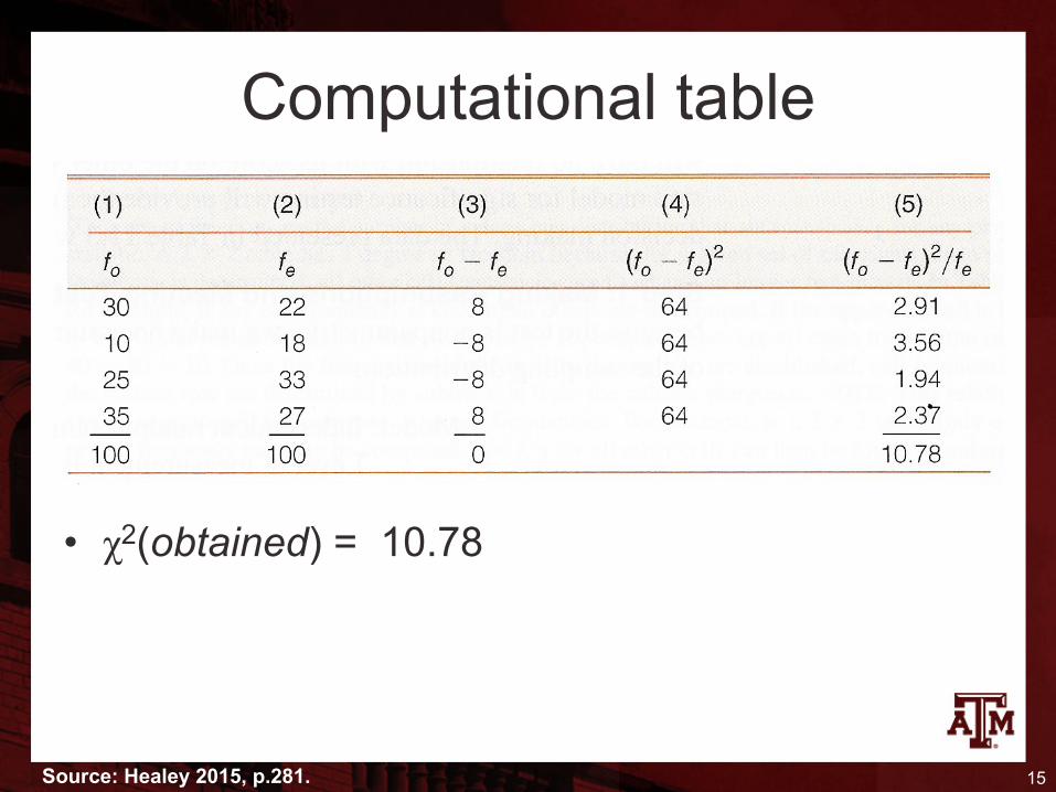
Computational table

15Source: Healey 2015, p.281.

• χ2(obtained) = 10.78

Step 5: Decision, interpret

16

• χ2(obtained) = 10.78– This is beyond χ2(critical) = 3.841– The obtained χ2 score falls in the critical region, so we reject the H0

– Therefore, the H0 is false and must be rejected

• There is a significant relationship between employment status and accreditation status in the population from which the sample was drawn

Interpreting chi square• The chi square test tells us only if the variables

are independent or not• It does not tell us the pattern or nature of the

relationship• To investigate the pattern, compute percentages

within each column and compare across the columns

17

Pearson chi2(4) = 1.3515 Pr = 0.853

100.00 100.00 100.00 Total 819 1,026 1,845 19.05 19.69 19.40 reduced a lot 156 202 358 22.10 23.20 22.71 reduced a little 181 238 419 40.17 40.25 40.22 remain the same as it 329 413 742 12.70 11.11 11.82 increased a little 104 114 218 5.98 5.75 5.85 increased a lot 49 59 108 should be male female Total to america nowadays respondents sex number of immigrants

column percentage frequency Key

. tab letin1 sex if year==2016, chi col

• Is opinion about immigration different by sex?

• The probability of not rejecting H0 is big (p>0.05)– Opinion about

immigration does not depend on respondent’s sex

GSS example

18

Source: 2016 General Social Survey.

Edited table

19

Opinion AboutNumber of Immigrants

Male(%)

Female(%)

Total(%)

Chi Square(df = 4) p-value

2004 2.3397 0.6740Increase a lot 3.17 4.30 3.78Increase a little 6.89 6.27 6.56Remain the same 35.01 34.05 34.49Reduce a little 27.68 28.72 28.24Reduce a lot 27.24 26.66 26.93Total(sample size)

100.00(914)

100.00(1,069)

100.00(1,983)

2010 7.0998 0.1310Increase a lot 5.21 3.88 4.45Increase a little 7.90 11.40 9.91Remain the same 35.29 34.96 35.10Reduce a little 24.03 25.31 24.77Reduce a lot 27.56 24.44 25.77Total(sample size)

100.00(595)

100.00(798)

100.00(1,393)

2016 1.3515 0.8530Increase a lot 5.98 5.75 5.85Increase a little 12.70 11.11 11.82Remain the same 40.17 40.25 40.22Reduce a little 22.10 23.20 22.71Reduce a lot 19.05 19.69 19.40Total(sample size)

100.00(819)

100.00(1,026)

100.00(1,845)

Source: 2004, 2010, 2016 General Social Surveys.

Table 1. Opinion of the U.S. adult population about how should the number of immigrants to the country be nowadays by sex, 2004, 2010, and 2016

Limitations of chi square• Difficult to interpret

– When variables have many categories– Best when variables have four or fewer categories

• With small sample size– We cannot assume that chi square sampling distribution will be

accurate– Small samples: High percentage of cells have expected

frequencies of 5 or less

• Like all tests of hypotheses– Chi square is sensitive to sample size– As N increases, obtained chi square increases– Large samples: Trivial relationships may be significant

• Statistical significance is not the same as substantive significance (importance, magnitude)

20