9/13/2016 1 Lecture 19 Slide 1 EE 5303 Electromagnetic Analysis Using Finite‐Difference Time‐Domain Lecture #19 Periodic Structures in FDTD These notes may contain copyrighted material obtained under fair use rules. Distribution of these materials is strictly prohibited Lecture Outline Lecture 19 Slide 2 • Review of Lecture 18 • Periodic Structures • Periodic Boundary Conditions in FDTD • Electromagnetic Band Calculation using FDTD
Transcript
9/13/2016
1
Lecture 19 Slide 1
EE 5303
Electromagnetic Analysis Using Finite‐Difference Time‐Domain
Lecture #19
Periodic Structures in FDTD These notes may contain copyrighted material obtained under fair use rules. Distribution of these materials is strictly prohibited
Lecture Outline
Lecture 19 Slide 2
• Review of Lecture 18
• Periodic Structures
• Periodic Boundary Conditions in FDTD
• Electromagnetic Band Calculation using FDTD
9/13/2016
2
Lecture 19 Slide 3
Review of Lecture 18
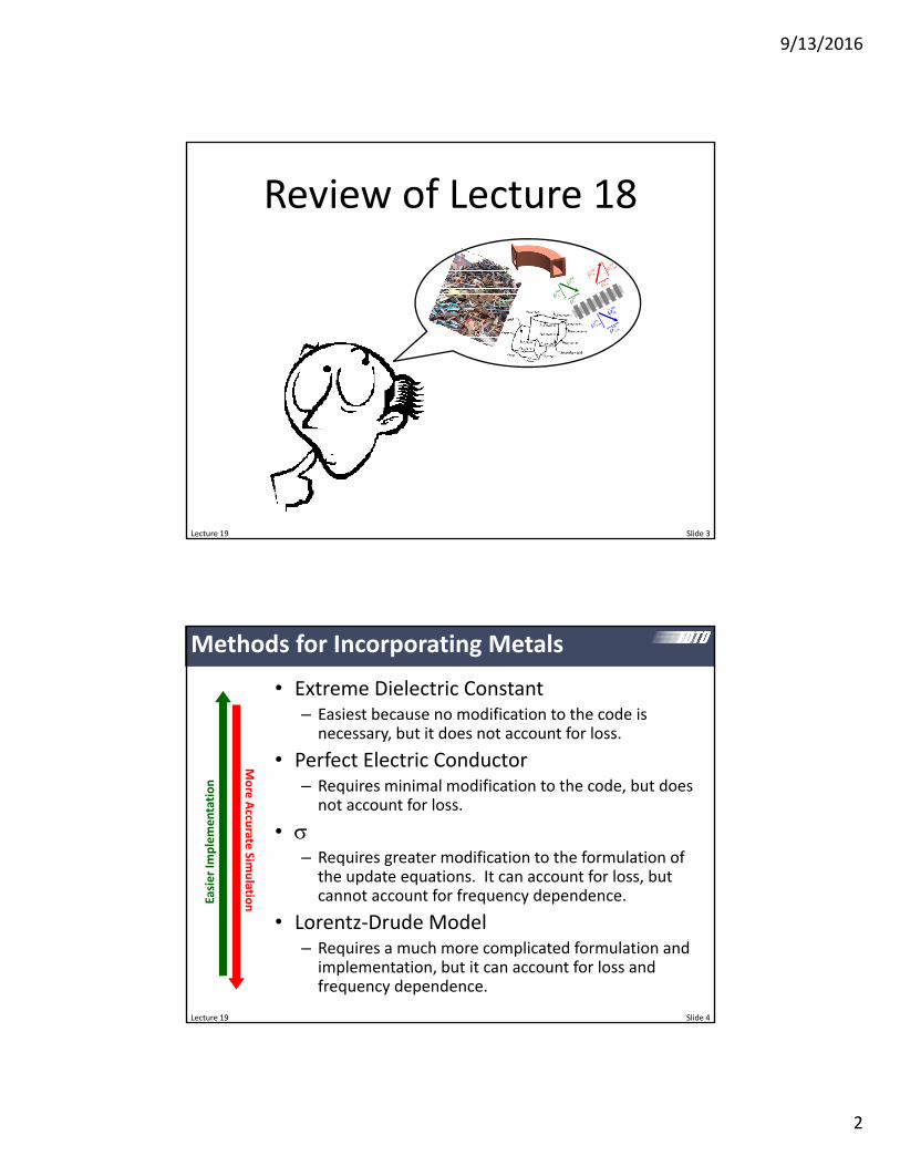
Methods for Incorporating Metals
• Extreme Dielectric Constant– Easiest because no modification to the code is necessary, but it does not account for loss.
• Perfect Electric Conductor– Requires minimal modification to the code, but does not account for loss.
• – Requires greater modification to the formulation of the update equations. It can account for loss, but cannot account for frequency dependence.
• Lorentz‐Drude Model– Requires a much more complicated formulation and implementation, but it can account for loss and frequency dependence.
Lecture 19 Slide 4
Easier Im
plementation
More Accu
rate Sim
ulatio
n
9/13/2016
3
Lecture 19 Slide 5
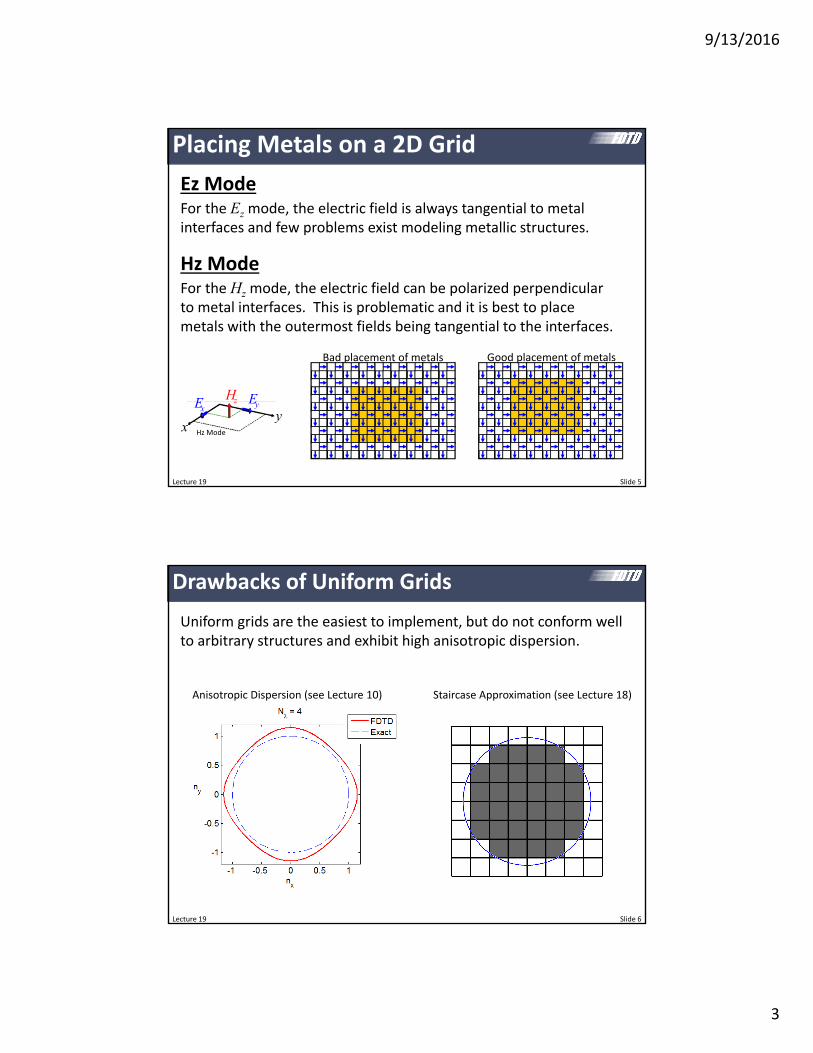
Placing Metals on a 2D Grid
Ez Mode
xy
zH yExE
Hz Mode
Bad placement of metals Good placement of metals
For the Ezmode, the electric field is always tangential to metal interfaces and few problems exist modeling metallic structures.
Hz ModeFor the Hzmode, the electric field can be polarized perpendicular to metal interfaces. This is problematic and it is best to place metals with the outermost fields being tangential to the interfaces.
Lecture 19 Slide 6
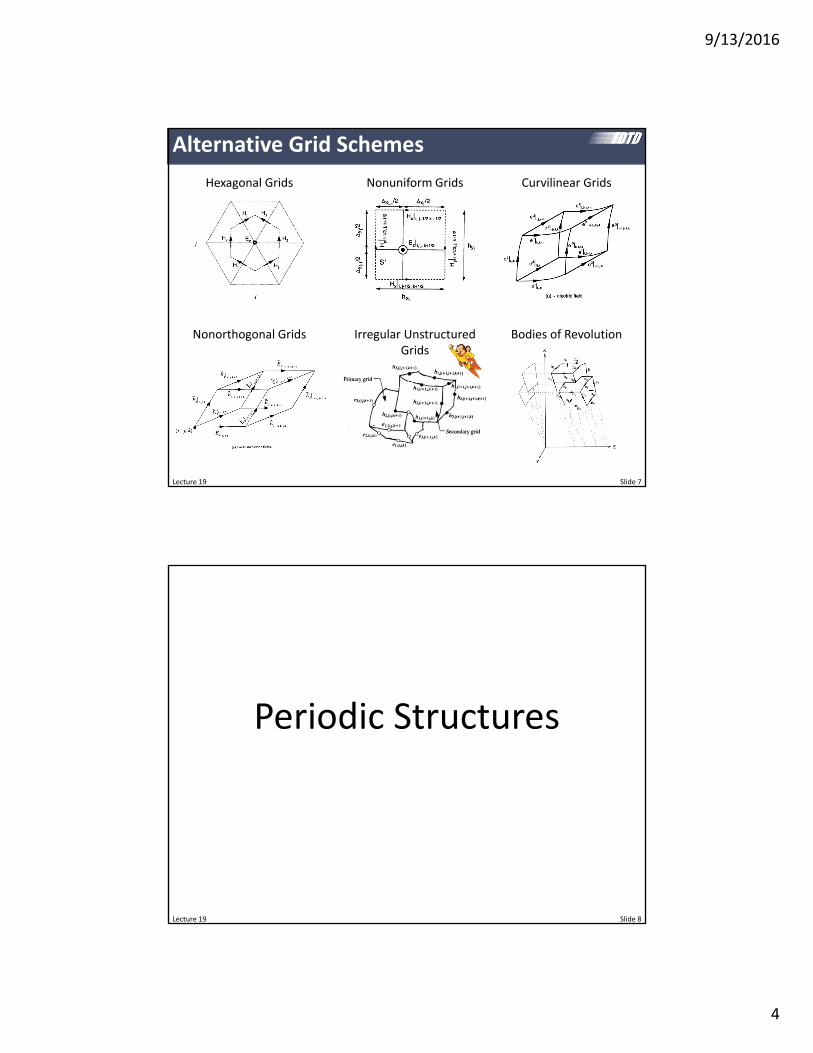
Drawbacks of Uniform Grids
Uniform grids are the easiest to implement, but do not conform well to arbitrary structures and exhibit high anisotropic dispersion.
Anisotropic Dispersion (see Lecture 10) Staircase Approximation (see Lecture 18)
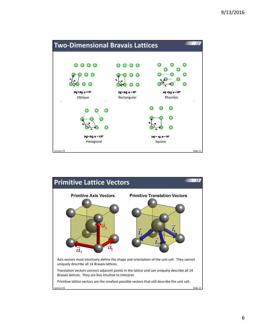
Axis vectors most intuitively define the shape and orientation of the unit cell. They cannot uniquely describe all 14 Bravais lattices.
Translation vectors connect adjacent points in the lattice and can uniquely describe all 14 Bravais lattices. They are less intuitive to interpret.
Primitive lattice vectors are the smallest possible vectors that still describe the unit cell.
9/13/2016
7
Lecture 19 Slide 13
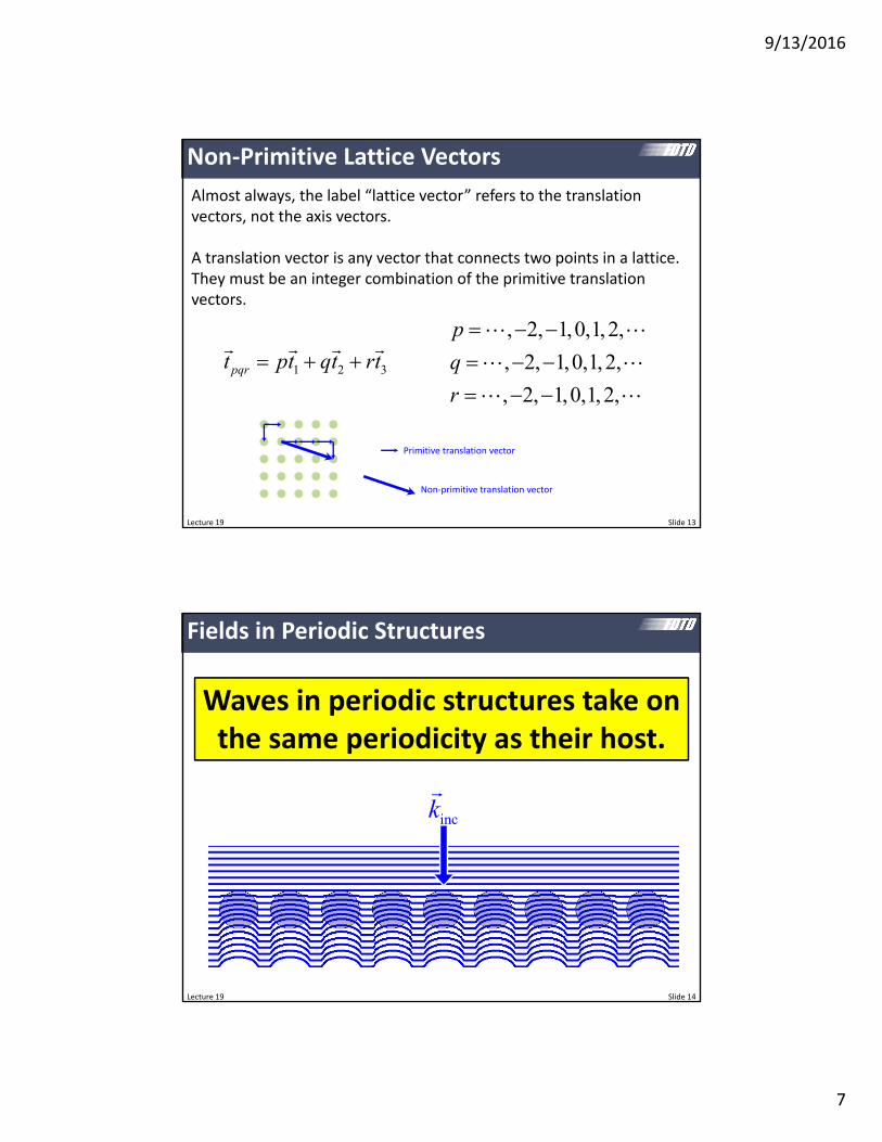
Non‐Primitive Lattice Vectors
Almost always, the label “lattice vector” refers to the translation vectors, not the axis vectors.
A translation vector is any vector that connects two points in a lattice. They must be an integer combination of the primitive translation vectors.
1 2 3pqrt pt qt rt
, 2, 1,0,1, 2,
, 2, 1,0,1,2,
, 2, 1,0,1, 2,
p
q
r
Primitive translation vector
Non‐primitive translation vector
Lecture 19 Slide 14
Fields in Periodic Structures
Waves in periodic structures take on the same periodicity as their host.Waves in periodic structures take on the same periodicity as their host.
inck
9/13/2016
8
Lecture 19 Slide 15
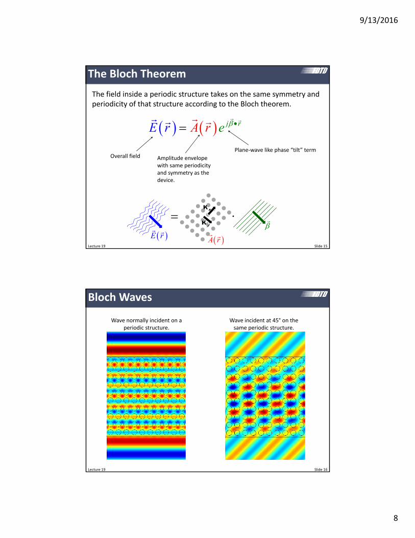
The Bloch Theorem
The field inside a periodic structure takes on the same symmetry and periodicity of that structure according to the Bloch theorem.
j rA r eE r
Overall field Amplitude envelope with same periodicity and symmetry as the device.
Plane‐wave like phase “tilt” term
A r E r
Lecture 19 Slide 16
Bloch Waves
Wave normally incident on a periodic structure.
Wave incident at 45° on the same periodic structure.
9/13/2016
9
Lecture 19 Slide 17
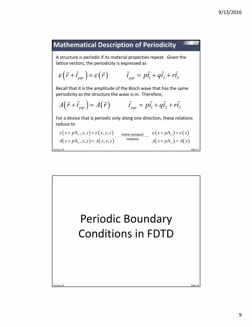
Mathematical Description of Periodicity
A structure is periodic if its material properties repeat. Given the lattice vectors, the periodicity is expressed as
1 2 3 pqr pqrr t r t pt qt rt
Recall that it is the amplitude of the Bloch wave that has the same periodicity as the structure the wave is in. Therefore,
1 2 3 pqr pqrA r t A r t pt qt rt
For a device that is periodic only along one direction, these relations reduce to
, , , ,
, , , ,
x
x
x p y z x y z
A x p y z A x y z
x
x
x p x
A x p A x
more compact
notation
Lecture 19 Slide 18
Periodic Boundary Conditions in FDTD
9/13/2016
10
Lecture 19 Slide 19
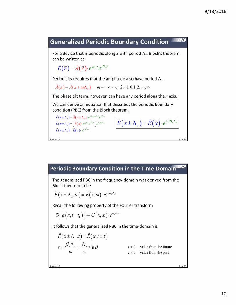
Generalized Periodic Boundary Condition
For a device that is periodic along x with period x, Bloch’s theorem can be written as
yxj yj xeA r eE r
Periodicity requires that the amplitude also have period x.
, , 2, 1,0,1,2, ,x mA x A x m
The phase tilt term, however, can have any period along the x axis.
We can derive an equation that describes the periodic boundary condition (PBC) from the Bloch theorem.
yx x
yx x x
x x
xx
x
x
j yj x
j yj x j
j
e e
e e
E x
E x
E x E x
A x
eA x
e
x xj
xE x E x e
Lecture 19 Slide 20
Periodic Boundary Condition in the Time‐Domain
The generalized PBC in the frequency‐domain was derived from the Bloch theorem to be
, , x xjxE x E x e
Recall the following property of the Fourier transform
00, , j tg x t t G x e
It follows that the generalized PBC in the time‐domain is
0
, ,
sin
x
x x x
E x t E x t
c
0 value from the future
0 value from the past
9/13/2016
11
Lecture 19 Slide 21
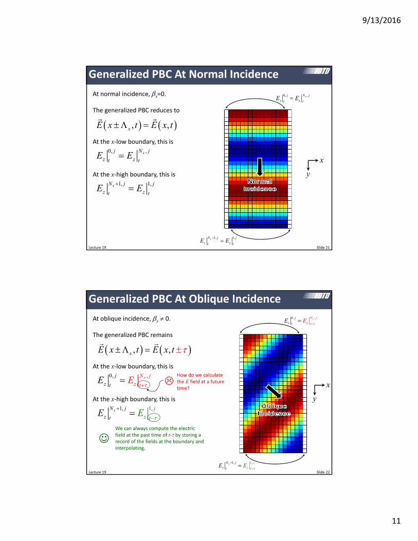
Generalized PBC At Normal Incidence
At normal incidence, x=0.
The generalized PBC reduces to
, ,xE x t E x t
At the x‐low boundary, this is0, ,xj N j
z zt tE E
At the x‐high boundary, this is1, 1,xN j j
z zt tE E
0, ,xj N j
z zt tE E
1, 1,xN j j
z zt tE E
x
y
Lecture 19 Slide 22
Generalized PBC At Oblique Incidence
At oblique incidence, x 0.
The generalized PBC remains
, ,xE x t E x t
At the x‐low boundary, this is
At the x‐high boundary, this is
0, ,xN j
z
j
t tzE E
1 1,,xN j j
z tz tEE
We can always compute the electric field at the past time of t‐ by storing a record of the fields at the boundary and interpolating.
How do we calculate the E field at a future time?
0, ,xN j
z
j
t tzE E
1 1,,xN j j
z tz tEE
x
y
9/13/2016
12
Conclusions
• Time‐domain methods have serious problems when the following conditions exist simultaneously– Periodic boundary condition
– Oblique incidence
– Pulsed source
• Good solutions exist when any one of these conditions can be removed.
• One limited solution exists when all of these conditions exist at the same time.– Angled‐update method
Lecture 19 Slide 23
Lecture 19 Slide 24
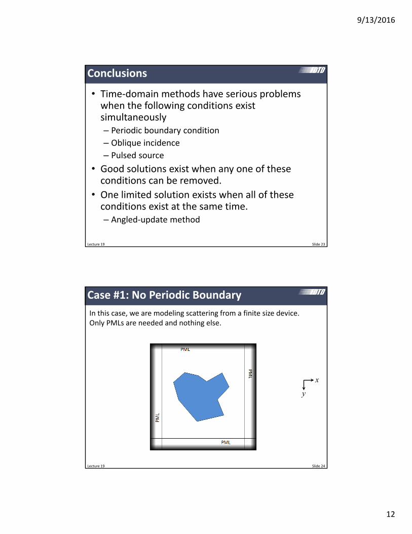
Case #1: No Periodic Boundary
In this case, we are modeling scattering from a finite size device. Only PMLs are needed and nothing else.
x
y
9/13/2016
13
Lecture 19 Slide 25
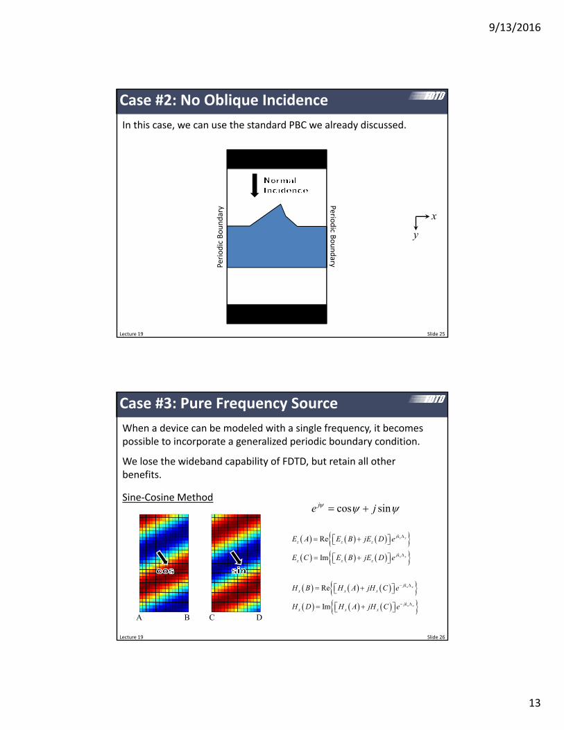
Case #2: No Oblique Incidence
In this case, we can use the standard PBC we already discussed.
Periodic Boundary
Perio
dic B
oundary
PML
PML
x
y
Lecture 19 Slide 26
Case #3: Pure Frequency Source
When a device can be modeled with a single frequency, it becomes possible to incorporate a generalized periodic boundary condition.
We lose the wideband capability of FDTD, but retain all other benefits.
Sine‐Cosine Method
Re
Im
Re
Im
x x
x x
x x
x x
jkz z z
jkz z z
jkx x x
jkx x x
E A E B jE D e
E C E B jE D e
H B H A jH C e
H D H A jH C e
A B C D
cos sinje j
9/13/2016
14
Lecture 19 Slide 27
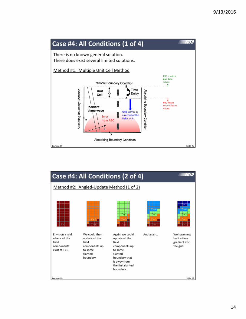
Case #4: All Conditions (1 of 4)
There is no known general solution. There does exist several limited solutions.
Method #1: Multiple Unit Cell Method
Grid serves as a record of the fields at A
PBC would require future values.
PBC requires past time values
Error from ABC
Lecture 19 Slide 28
Case #4: All Conditions (2 of 4)
Method #2: Angled‐Update Method (1 of 2)
1T
Envision a grid where all the field components exist at T=1.
1T
2T
We could then update all the field components up to some slanted boundary.
1T
2T
3T
Again, we could update all the field components up to some slanted boundary that is away from the first slanted boundary.
1T
2T
3T
4T
And again…
1T
2T
3T
4T
5T
We have now built a time gradient into the grid.
9/13/2016
15
Lecture 19 Slide 29
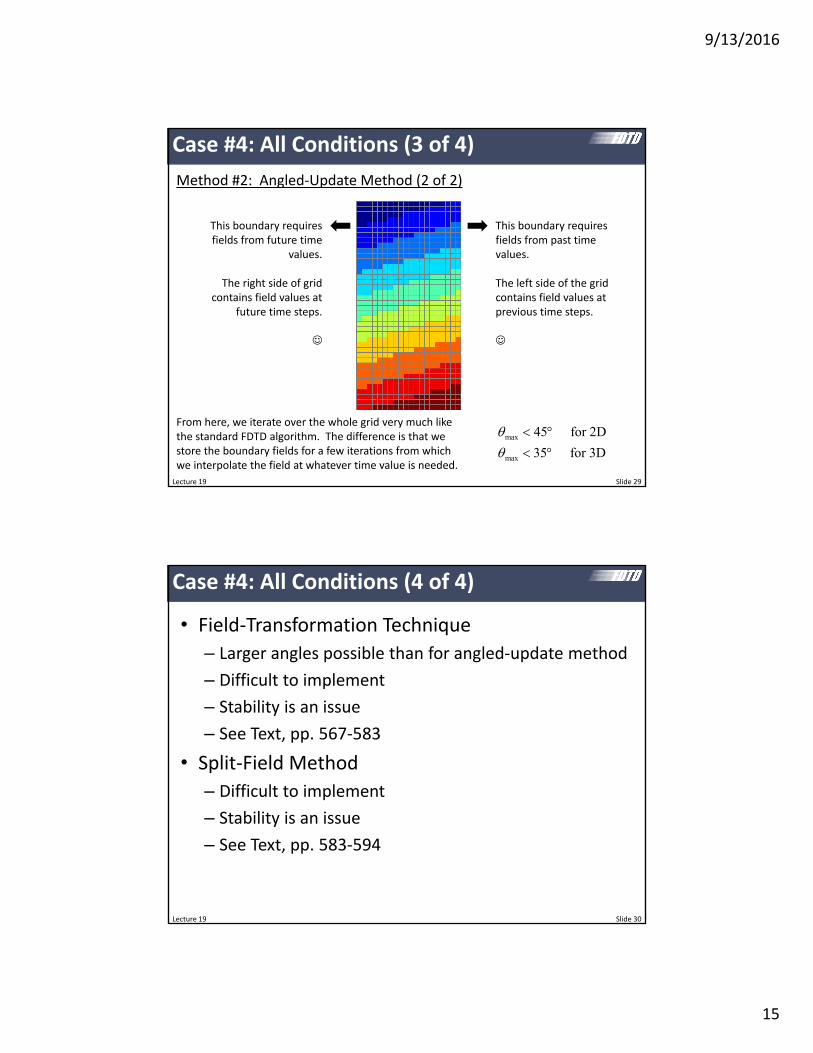
Case #4: All Conditions (3 of 4)
Method #2: Angled‐Update Method (2 of 2)
This boundary requires fields from past time values.
The left side of the grid contains field values at previous time steps.
This boundary requires fields from future time
values.
The right side of grid contains field values at
future time steps.
From here, we iterate over the whole grid very much like the standard FDTD algorithm. The difference is that we store the boundary fields for a few iterations from which we interpolate the field at whatever time value is needed.
max
max
45 for 2D
35 for 3D
Case #4: All Conditions (4 of 4)
• Field‐Transformation Technique
– Larger angles possible than for angled‐update method
– Difficult to implement
– Stability is an issue
– See Text, pp. 567‐583
• Split‐Field Method
– Difficult to implement
– Stability is an issue
– See Text, pp. 583‐594
Lecture 19 Slide 30
9/13/2016
16
Lecture 19 Slide 31
Electromagnetic Band Calculation using FDTD
Lecture 19 Slide 32
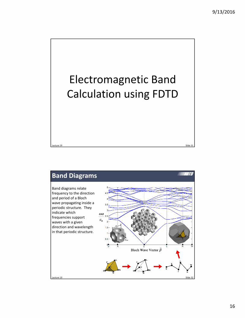
Band Diagrams
Band diagrams relate frequency to the direction and period of a Bloch wave propagating inside a periodic structure. They indicate which frequencies support waves with a given direction and wavelength in that periodic structure.
9/13/2016
17
Lecture 19 Slide 33
Computation of Band Diagrams
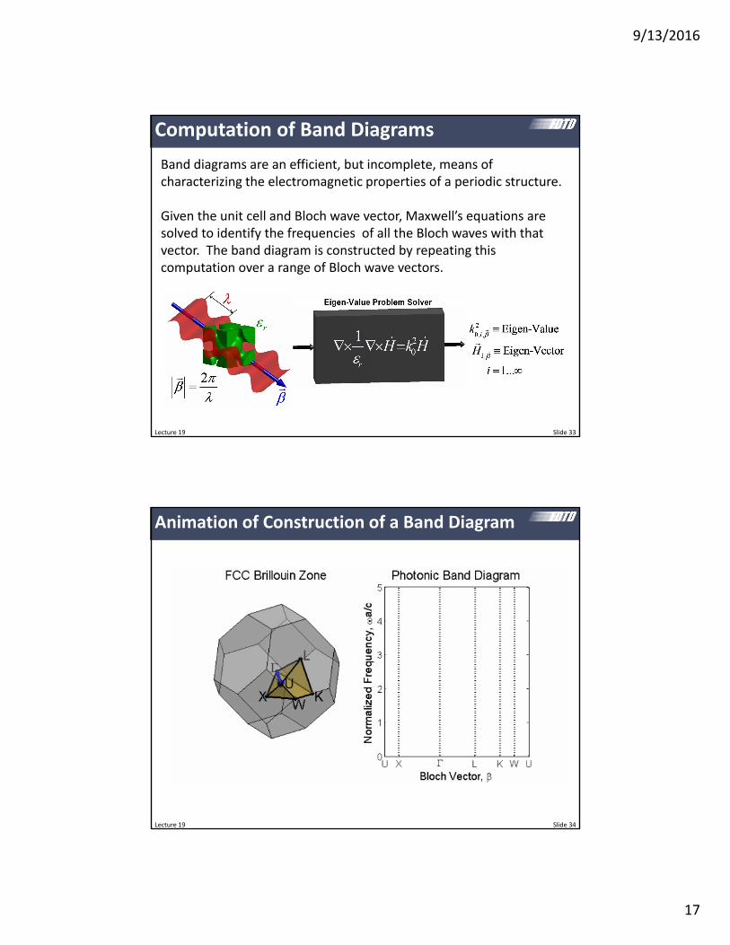
Band diagrams are an efficient, but incomplete, means of characterizing the electromagnetic properties of a periodic structure.
Given the unit cell and Bloch wave vector, Maxwell’s equations are solved to identify the frequencies of all the Bloch waves with that vector. The band diagram is constructed by repeating this computation over a range of Bloch wave vectors.
Lecture 19 Slide 34
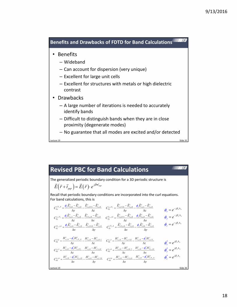
Animation of Construction of a Band Diagram
9/13/2016
18
Benefits and Drawbacks of FDTD for Band Calculations
• Benefits
– Wideband
– Can account for dispersion (very unique)
– Excellent for large unit cells
– Excellent for structures with metals or high dielectric contrast
• Drawbacks
– A large number of iterations is needed to accurately identify bands
– Difficult to distinguish bands when they are in close proximity (degenerate modes)
– No guarantee that all modes are excited and/or detected
Lecture 19 Slide 35
Lecture 19 Slide 36
Revised PBC for Band Calculations
The generalized periodic boundary condition for a 3D periodic structure is
Recall that periodic boundary conditions are incorporated into the curl equations. For band calculations, this is
pqrj t
pqrE r t E r e
, , ,1, , , , , 1 , , , 1, , , , ,1 , ,, ,
, ,1 , , 1, , , , , , 1 , ,, ,, ,
y z
xz
z z y y z z y yi N k i k i j k i j k i j k i j k i j k i j i j ki j NEx Ex
x x z z x xi j i j k i j k i j k i j k i j
y
kN j ki j NEy Ey
z
z
E E E E E E E EC C
y z y z
E E E E E EC C
z x z
1, , , ,
, ,1, , , , , 1, , , 1, , , , ,1, , ,, , yx
z zj k i j k
y y x x y y x xi N kj k i j k i j k i j k i j k i j k i k i j kN j k
Ez Ez
x
x y
E E
x
E E E E E E E EC C
x y x y
, , , , , , , ,, , , , 1 , , , 1,,1, , ,1
, ,, , , , , , 1, , , , , , 1, ,1 1
*
,
*
*,
*
y z
z
z z y yy y z zi j k i N k i j k i j Ni j k i j k i j k i j ki k i j
Hx Hx
zx x z z x xi j ki j k i j N i j k i j k i j k i j ki j j k
Hy H
y
y
z
xz
H H H HH H H HC C
y z y z
HH H H H H HC C
z x z
, ,
, , , ,, , , , , , , 1, , , 1, ,1, 1
**, , ,
x
yx
zN j k
x xy y x x y yi j k i N ki j k N j k i j k i j k i j k i j kj k i k
H
y
z Hzx
H
x
H HH H H H H HC C
x y x y
x x
y y
z z
j
j
x
zj
y
e
e
e
*
*
*
x x
y y
z z
j
j
x
y
zj
e
e
e
9/13/2016
19
Lecture 19 Slide 37
Implementation of PBC in MATLAB
, , , , , , , 1,1, ,
, , , ,, , 1, ,,1,
*
*
x
y
y y x xi j k N j k i j k i j kj k
Hz
x xy yi j k i N ki j k i j ki k
Hz
x
y
H H H HC
x y
H HH HC
x y
x x
y y
jx
yj
e
e
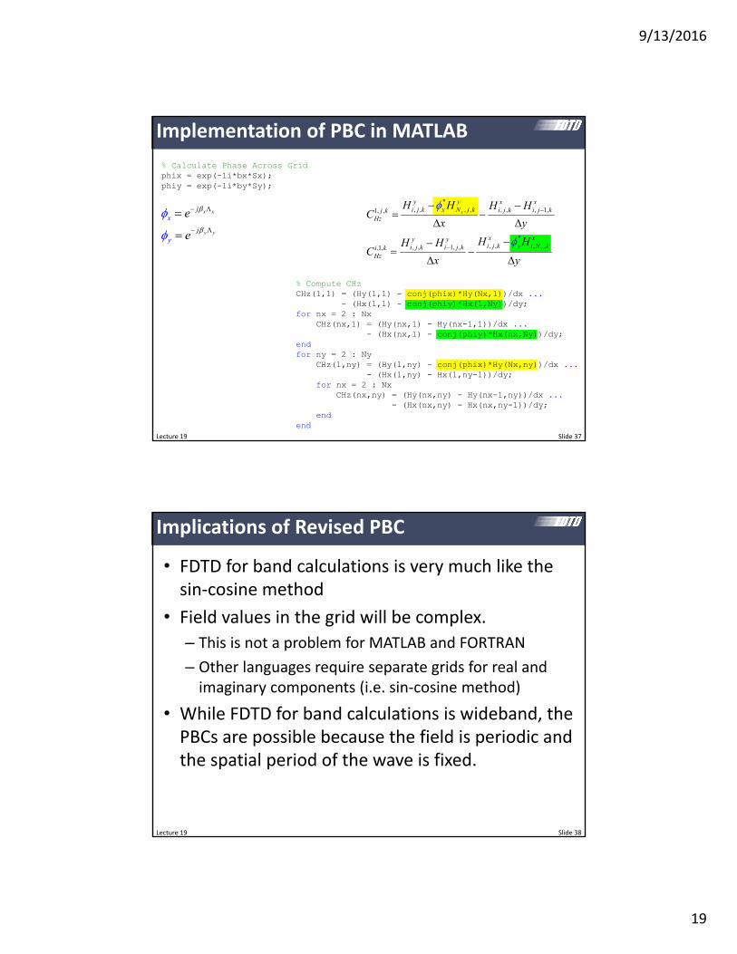
% Calculate Phase Across Gridphix = exp(-1i*bx*Sx);phiy = exp(-1i*by*Sy);
• FDTD for band calculations is very much like the sin‐cosine method
• Field values in the grid will be complex.
– This is not a problem for MATLAB and FORTRAN
– Other languages require separate grids for real and imaginary components (i.e. sin‐cosine method)
• While FDTD for band calculations is wideband, the PBCs are possible because the field is periodic and the spatial period of the wave is fixed.
Lecture 19 Slide 38
9/13/2016
20
Lecture 19 Slide 39
The Source
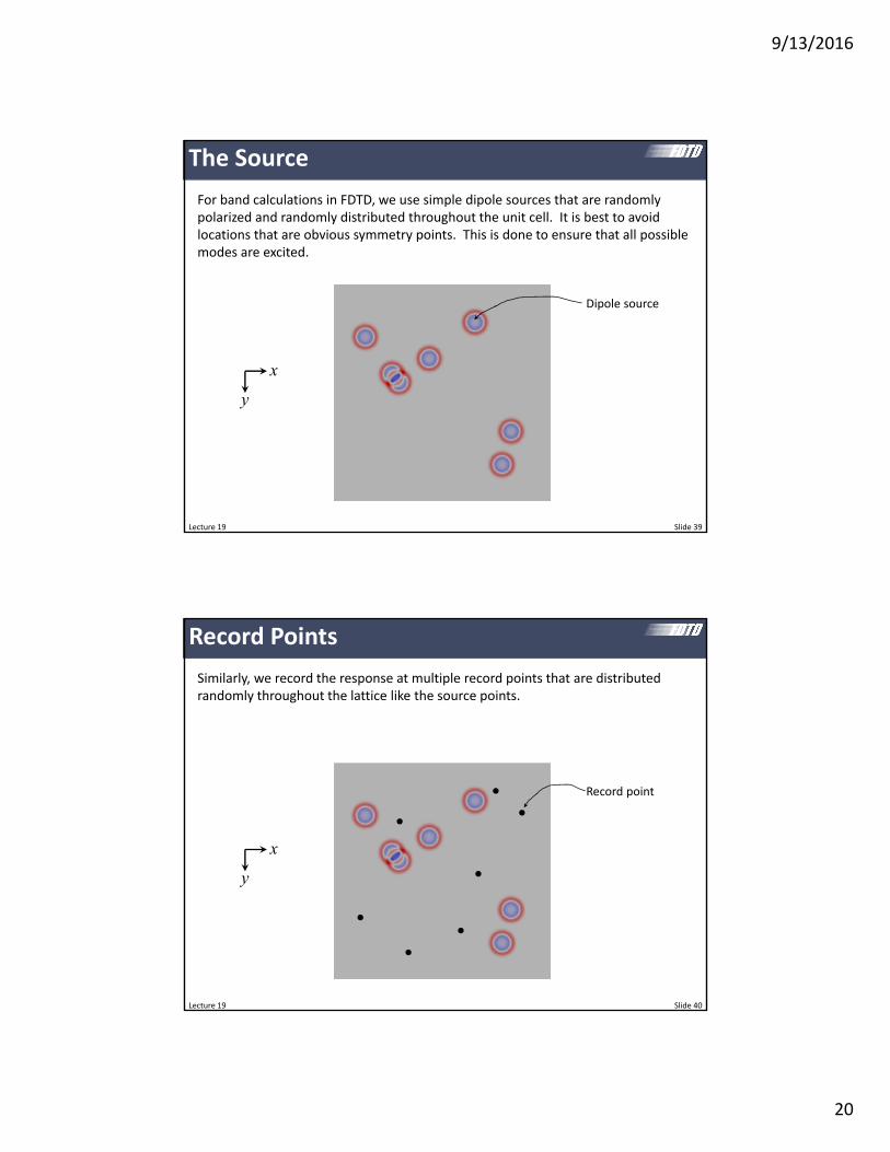
For band calculations in FDTD, we use simple dipole sources that are randomly polarized and randomly distributed throughout the unit cell. It is best to avoid locations that are obvious symmetry points. This is done to ensure that all possible modes are excited.
Dipole source
x
y
Lecture 19 Slide 40
Record Points
Similarly, we record the response at multiple record points that are distributed randomly throughout the lattice like the source points.
Record point
x
y
9/13/2016
21
Lecture 19 Slide 41
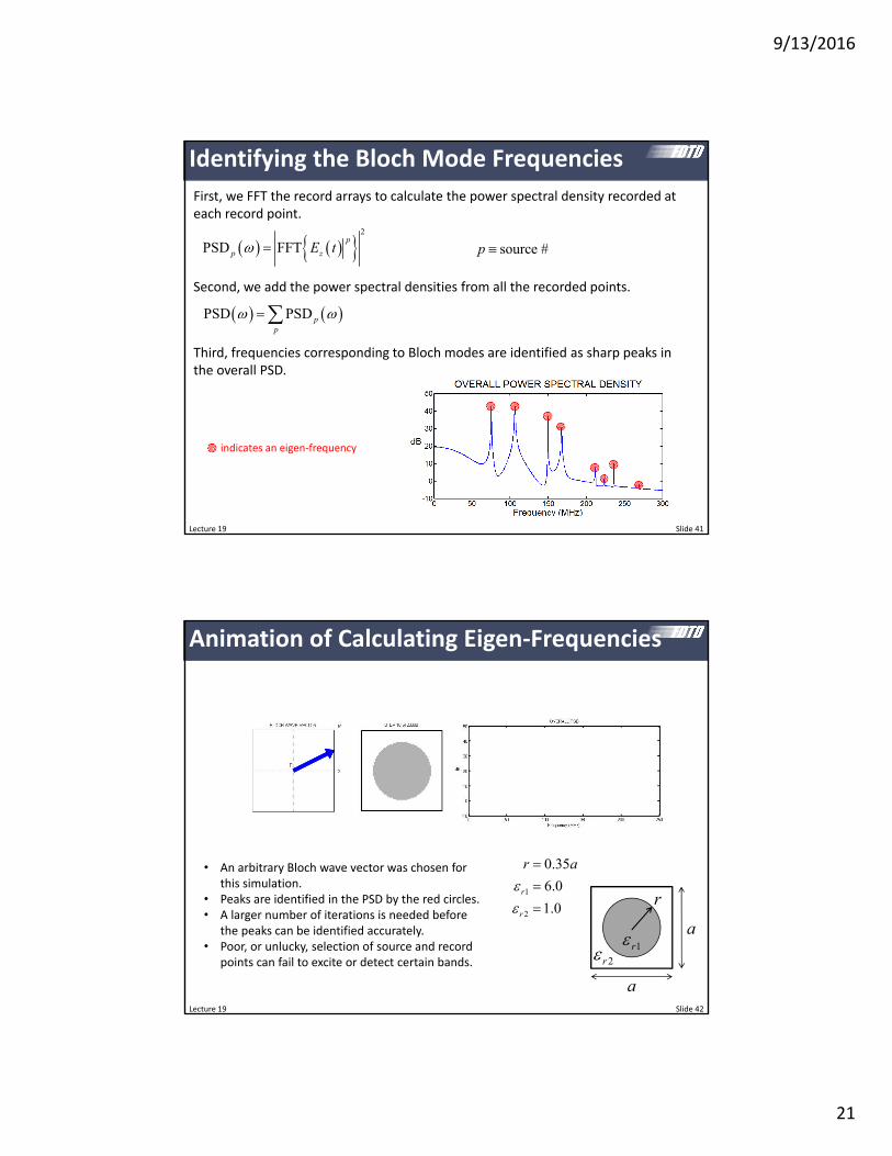
Identifying the Bloch Mode Frequencies
First, we FFT the record arrays to calculate the power spectral density recorded at each record point.
2
PSD FFTp
p zE t
Second, we add the power spectral densities from all the recorded points.
PSD PSD pp
Third, frequencies corresponding to Bloch modes are identified as sharp peaks in the overall PSD.
indicates an eigen‐frequency
source #p
Lecture 19 Slide 42
Animation of Calculating Eigen‐Frequencies
• An arbitrary Bloch wave vector was chosen for this simulation.
• Peaks are identified in the PSD by the red circles.• A larger number of iterations is needed before
the peaks can be identified accurately.• Poor, or unlucky, selection of source and record
points can fail to excite or detect certain bands.
a
a
r
1r2r
1
2
0.35
6.0
1.0r
r
r a
9/13/2016
22
Lecture 19 Slide 43
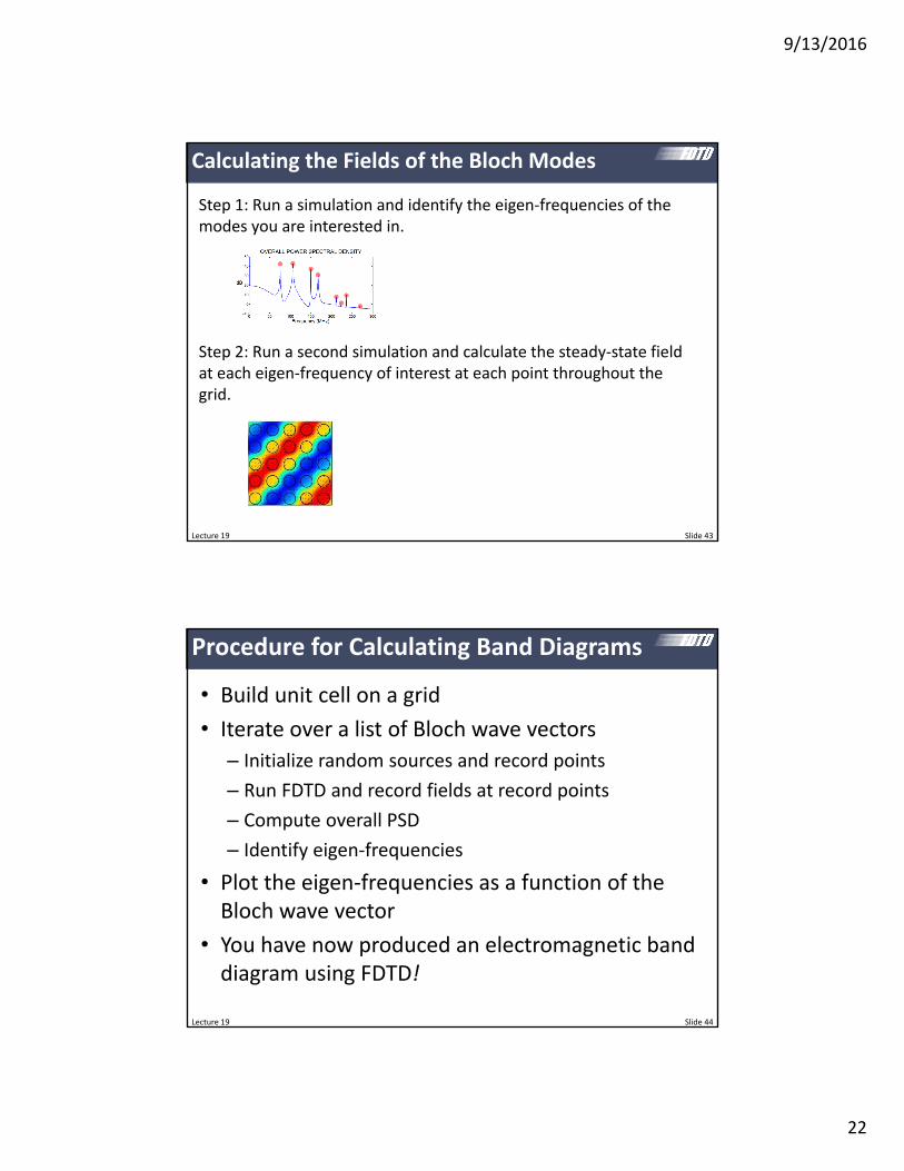
Calculating the Fields of the Bloch Modes
Step 1: Run a simulation and identify the eigen‐frequencies of the modes you are interested in.
Step 2: Run a second simulation and calculate the steady‐state field at each eigen‐frequency of interest at each point throughout the grid.
Procedure for Calculating Band Diagrams
• Build unit cell on a grid
• Iterate over a list of Bloch wave vectors
– Initialize random sources and record points
– Run FDTD and record fields at record points
– Compute overall PSD
– Identify eigen‐frequencies
• Plot the eigen‐frequencies as a function of the Bloch wave vector
• You have now produced an electromagnetic band diagram using FDTD!
Lecture 19 Slide 44
9/13/2016
23
Lecture 19 Slide 45
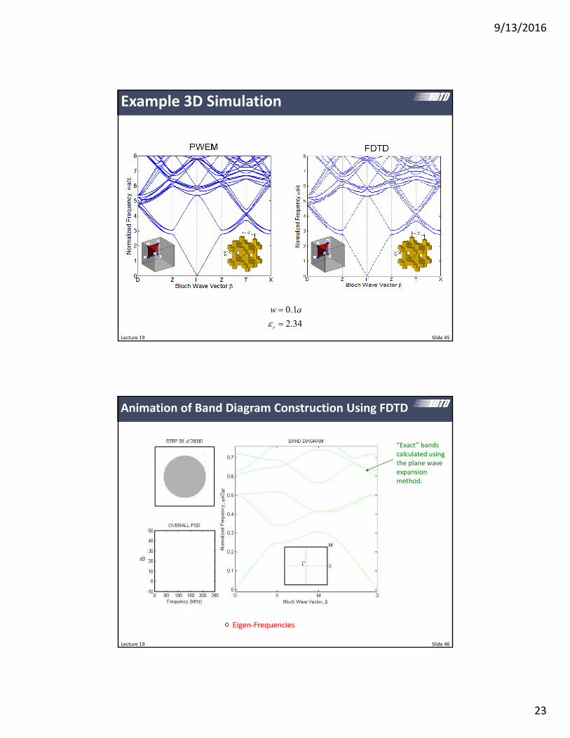
Example 3D Simulation
0.1
2.34r
w a
Lecture 19 Slide 46
Animation of Band Diagram Construction Using FDTD
“Exact” bands calculated using the plane wave expansion method.