11/12/12 1 Bayes Theorem Regression Analysis Chapter 2 (Chines version only) Lecture 2 To accompany Quantitative Analysis for Management, Eleventh Edition, by Render, Stair, and Hanna Power Point slides created by Brian Peterson Today’s lecture Textbook Chapter 2 and 4 Bayes Theorem & Regression Analysis 1-2 Today’s tutorial Review of today’s lecture; Practice calculations; Introduction Life is uncertain; we are not sure what the future will bring. Probability is a numerical statement about the likelihood that an event will occur. 2-3 Fundamental Concepts 1. The probability, P, of any event or state of nature occurring is greater than or equal to 0 and less than or equal to 1. That is: 0 ≤ P (event) ≤ 1 2. The sum of the simple probabilities for all possible outcomes of an activity must equal 1. 2-4 Chapters in This Book That Use Probability 2-5 CHAPTER TITLE 3 Decision Analysis 4 Regression Models 5 Forecasting 6 Inventory Control Models 12 Project Management 13 Waiting Lines and Queuing Theory Models 14 Simulation Modeling 15 Markov Analysis 16 Statistical Quality Control Module 3 Decision Theory and the Normal Distribution Module 4 Game Theory Table 2.1 Diversey Paint Example Demand for white latex paint at Diversey Paint and Supply has always been either 0, 1, 2, 3, or 4 gallons per day. Over the past 200 days, the owner has observed the following frequencies of demand: 2-6 QUANTITY DEMANDED NUMBER OF DAYS PROBABILITY 0 40 0.20 (= 40/200) 1 80 0.40 (= 80/200) 2 50 0.25 (= 50/200) 3 20 0.10 (= 20/200) 4 10 0.05 (= 10/200) Total 200 Total 1.00 (= 200/200)
Transcript
11/12/12
1
Bayes Theorem Regression Analysis
Chapter 2 (Chines version only)
Lecture 2
To accompany Quantitative Analysis for Management, Eleventh Edition, by Render, Stair, and Hanna Power Point slides created by Brian Peterson
Today’s tutorial § Review of today’s lecture; § Practice calculations;
Introduction
n Life is uncertain; we are not sure what the future will bring. n Probability is a numerical statement about the likelihood that an event will occur.
2-3
Fundamental Concepts
1. The probability, P, of any event or state of nature occurring is greater than or equal to 0 and less than or equal to 1. That is:
0 ≤ P (event) ≤ 1
2. The sum of the simple probabilities for all possible outcomes of an activity must equal 1.
2-4
Chapters in This Book That Use Probability
2-5
CHAPTER TITLE 3 Decision Analysis 4 Regression Models 5 Forecasting 6 Inventory Control Models 12 Project Management 13 Waiting Lines and Queuing Theory Models 14 Simulation Modeling 15 Markov Analysis 16 Statistical Quality Control Module 3 Decision Theory and the Normal Distribution Module 4 Game Theory
Table 2.1
Diversey Paint Example
§ Demand for white latex paint at Diversey Paint and Supply has always been either 0, 1, 2, 3, or 4 gallons per day.
§ Over the past 200 days, the owner has observed the following frequencies of demand:
The equation must be modified to account for double counting.
n The probability is reduced by subtracting the chance of both events occurring together.
Venn Diagrams
2-16
P (A) P (B)
Events that are mutually exclusive.
P (A or B) = P (A) + P (B)
Figure 2.1
Events that are not mutually exclusive.
P (A or B) = P (A) + P (B) – P (A and B)
Figure 2.2
P (A) P (B)
P (A and B)
Statistically Independent Events
Events may be either independent or dependent.
– For independent events, the occurrence of one event has no effect on the probability of occurrence of the second event.
2-17
Which Sets of Events Are Independent?
2-18
1. (a) Your education (b) Your income level
2. (a) Draw a jack of hearts from a full 52-card deck (b) Draw a jack of clubs from a full 52-card deck
3. (a) Chicago Cubs win the National League pennant (b) Chicago Cubs win the World Series
4. (a) Snow in Santiago, Chile (b) Rain in Tel Aviv, Israel
Dependent events
Dependent events
Independent events
Independent events
11/12/12
4
Three Types of Probabilities n Marginal (or simple) probability is just the probability of a
single event occurring. P (A)
2-19
n Joint probability is the probability of two or more events occurring and is equal to the product of their marginal probabilities for independent events.
P (AB) = P (A) x P (B) n Conditional probability is the probability of event
B given that event A has occurred. P (B | A) = P (B)
n Or the probability of event A given that event B has occurred
P (A | B) = P (A)
Joint Probability Example
2-20
The probability of tossing a 6 on the first roll of the die and a 2 on the second roll:
P (6 on first and 2 on second) = P (tossing a 6) x P (tossing a 2) = 1/6 x 1/6 = 1/36 = 0.028
Independent Events
1. The probability of a black ball drawn on first draw is: P (B) = 0.30 (a marginal probability)
2. The probability of two green balls drawn is: P (GG) = P (G) x P (G) = 0.7 x 0.7 = 0.49 (a joint probability for two independent
events)
2-21
A bucket contains 3 black balls and 7 green balls. n Draw a ball from the bucket, replace it, and
draw a second ball.
Independent Events
3. The probability of a black ball drawn on the second draw if the first draw is green is:
P (B | G) = P (B) = 0.30 (a conditional probability but equal to the
marginal because the two draws are independent events)
4. The probability of a green ball drawn on the second draw if the first draw is green is:
P (G | G) = P (G) = 0.70 (a conditional probability as in event 3)
2-22
A bucket contains 3 black balls and 7 green balls. n Draw a ball from the bucket, replace it, and
draw a second ball.
Statistically Dependent Events The marginal probability of an event occurring is computed in the same way:
P (A)
2-23
The formula for the joint probability of two events is: P (AB) = P (B | A) P (A)
P (A | B) = P (AB) P (B)
Calculating conditional probabilities is slightly more complicated. The probability of event A given that event B has occurred is:
When Events Are Dependent
2-24
Assume that we have an urn containing 10 balls of the following descriptions: n 4 are white (W) and lettered (L) n 2 are white (W) and numbered (N) n 3 are yellow (Y) and lettered (L) n 1 is yellow (Y) and numbered (N)
P (WL) = 4/10 = 0.4 P (YL) = 3/10 = 0.3 P (WN) = 2/10 = 0.2 P (YN) = 1/10 = 0.1 P (W) = 6/10 = 0.6 P (L) = 7/10 = 0.7 P (Y) = 4/10 = 0.4 P (N) = 3/10 = 0.3
11/12/12
5
When Events Are Dependent
2-25
4 balls White (W)
and Lettered (L)
2 balls White (W)
and Numbered (N)
3 balls Yellow (Y)
and Lettered (L)
1 ball Yellow (Y) and Numbered (N)
Probability (WL) = 4 10
Probability (YN) = 1 10
Probability (YL) = 3 10
Probability (WN) = 2 10
The urn contains 10 balls:
Figure 2.3
When Events Are Dependent
2-26
The conditional probability that the ball drawn is lettered, given that it is yellow, is:
P (L | Y) = = = 0.75 P (YL) P (Y)
0.3 0.4
We can verify P (YL) using the joint probability formula
P (YL) = P (L | Y) x P (Y) = (0.75)(0.4) = 0.3
Joint Probabilities for Dependent Events
P (MT) = P (T | M) x P (M) = (0.70)(0.40) = 0.28
2-27
If the stock market reaches 12,500 point by January, there is a 70% probability that Tubeless Electronics will go up.
n You believe that there is only a 40% chance the stock market will reach 12,500.
n Let M represent the event of the stock market reaching 12,500 and let T be the event that Tubeless goes up in value.
Revising Probabilities with Bayes’ Theorem
2-28
Posterior Probabilities
Bayes’ Process
Bayes’ theorem is used to incorporate additional information and help create posterior probabilities.
Prior Probabilities
New Information
Figure 2.4
Posterior Probabilities A cup contains two dice identical in appearance but one is fair (unbiased), the other is loaded (biased).
§ The probability of rolling a 3 on the fair die is 1/6 or 0.166. § The probability of tossing the same number on the loaded die
is 0.60. § We select one by chance,
toss it, and get a 3. § What is the probability that
the die rolled was fair? § What is the probability that
the loaded die was rolled?
2-29
Posterior Probabilities We know the probability of the die being fair or loaded is:
P (fair) = 0.50 P (loaded) = 0.50 And that
P (3 | fair) = 0.166 P (3 | loaded) = 0.60
2-30
We compute the probabilities of P (3 and fair) and P (3 and loaded):
P (3 and fair) = P (3 | fair) x P (fair) = (0.166)(0.50) = 0.083
P (3 and loaded) = P (3 | loaded) x P (loaded) = (0.60)(0.50) = 0.300
11/12/12
6
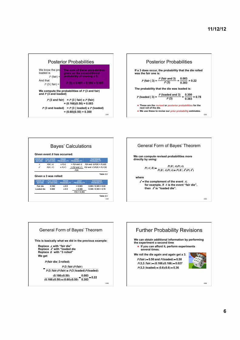
Posterior Probabilities We know the probability of the die being fair or loaded is
P (fair) = 0.50 P (loaded) = 0.50 And that
P (3 | fair) = 0.166 P (3 | loaded) = 0.60
2-31
We compute the probabilities of P (3 and fair) and P (3 and loaded)
P (3 and fair) = P (3 | fair) x P (fair) = (0.166)(0.50) = 0.083
P (3 and loaded) = P (3 | loaded) x P (loaded) = (0.60)(0.50) = 0.300
The sum of these probabilities gives us the unconditional probability of tossing a 3:
P (3) = 0.083 + 0.300 = 0.383
Posterior Probabilities
2-32
P (loaded | 3) = = = 0.78 P (loaded and 3)
P (3) 0.300 0.383
The probability that the die was loaded is:
P (fair | 3) = = = 0.22 P (fair and 3)
P (3) 0.083 0.383
If a 3 does occur, the probability that the die rolled was the fair one is:
n These are the revised or posterior probabilities for the next roll of the die.
n We use these to revise our prior probability estimates.
Bayes’ Calculations
2-33
Given event B has occurred: STATE OF NATURE
P (B | STATE OF NATURE)
PRIOR PROBABILITY
JOINT PROBABILITY
POSTERIOR PROBABILITY
A P(B | A) x P(A) = P(B and A) P(B and A)/P(B) = P(A|B) A’ P(B | A’) x P(A’) = P(B and A’) P(B and A’)/P(B) = P(A’|B)
P(B)
Table 2.2 Given a 3 was rolled:
STATE OF NATURE
P (B | STATE OF NATURE)
PRIOR PROBABILITY
JOINT PROBABILITY
POSTERIOR PROBABILITY
Fair die 0.166 x 0.5 = 0.083 0.083 / 0.383 = 0.22 Loaded die 0.600 x 0.5 = 0.300 0.300 / 0.383 = 0.78
P(3) = 0.383
Table 2.3
General Form of Bayes’ Theorem
2-34
)()|()()|()()|()|(
APABPAPABPAPABPBAP
ʹ′ʹ′+=
We can compute revised probabilities more directly by using:
where the complement of the event ; for example, if is the event “fair die”, then is “loaded die”.
AA
Aʹ′
= ʹ′ A
General Form of Bayes’ Theorem
2-35
This is basically what we did in the previous example:
Replace with “fair die” Replace with “loaded die Replace with “3 rolled” We get
AAʹ′B
)|( rolled 3die fairP
)()|()()|()()|(
loadedloaded3fairfair3fairfair3
PPPPPP
+=
22038300830
50060050016605001660 .
.
.).)(.().)(.(
).)(.(==
+
Further Probability Revisions
2-36
We can obtain additional information by performing the experiment a second time
n If you can afford it, perform experiments several times.
We roll the die again and again get a 3. 500loaded and 500fair .)(.)( == PP
3606060loaded33027016601660fair33
.).)(.()|,(.).)(.()|,(
==
==
PP
11/12/12
7
Further Probability Revisions
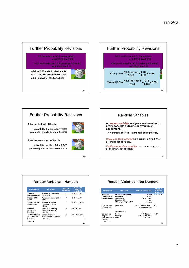
2-37
We can obtain additional information by performing the experiment a second time
n If you can afford it, perform experiments several times
We roll the die again and again get a 3 500loaded and 500fair .)(.)( == PP
3606060loaded33027016601660fair33
.).)(.()|,(.).)(.()|,(
==
==
PP
)()|,()( fairfair33fair and 3,3 PPP ×=0130500270 .).)(.( ==
)()|,()( loadedloaded33loaded and 3,3 PPP ×=18050360 .).)(.( ==
Further Probability Revisions
2-38
We can obtain additional information by performing the experiment a second time
n If you can afford it, perform experiments several times
We roll the die again and again get a 3 50.0)loaded( and 50.0)fair( == PP
Probability Distribution of a Discrete Random Variable
2-43
The students in Pat Shannon’s statistics class have just completed a quiz of five algebra problems. The distribution of correct scores is given in the following table:
For discrete random variables a probability is assigned to each event.
Probability Distribution of a Discrete Random Variable
The Probability Distribution follows all three rules: 1. Events are mutually exclusive and collectively exhaustive. 2. Individual probability values are between 0 and 1. 3. Total of all probability values equals 1.
Table 2.6
Probability Distribution for Dr. Shannon’s Class
2-45
P (X
)
0.4 –
0.3 –
0.2 –
0.1 –
0 – | | | | | | 1 2 3 4 5
X
Figure 2.5
Probability Distribution for Dr. Shannon’s Class
2-46
P (X
)
0.4 –
0.3 –
0.2 –
0.1 –
0 – | | | | | | 1 2 3 4 5
X
Figure 2.5
The central tendency of the distribution is the mean, or expected value. The amount of variability is the variance.
Expected Value of a Discrete Probability Distribution
2-47
( ) ( )∑=
=n
iii XPXXE
1
( ) )(...)( 2211 nn XPXXPXXPX +++=
The expected value is a measure of the central tendency of the distribution and is a weighted average of the values of the random variable.
where iX)( iXP
∑=
n
i 1)(XE
= random variable’s possible values = probability of each of the random variable’s
possible values = summation sign indicating we are adding all n
possible values = expected value or mean of the random sample
Expected Value of a Discrete Probability Distribution
2-48
( ) ( )∑=
=n
iii XPXXE
1
9.21.6.9.8.5.
)1.0(1)3.0(2)3.0(3)2.0(4)1.0(5
=
++++=
++++=
For Dr. Shannon’s class:
11/12/12
9
Variance of a Discrete Probability Distribution
2-49
For a discrete probability distribution the variance can be computed by
)()]([∑=
−==n
iii XPXEX
1
22 Varianceσ
where iX)(XE
)( iXP
= random variable’s possible values = expected value of the random variable = difference between each value of the random
variable and the expected mean = probability of each possible value of the
random variable
)]([ XEXi −
Variance of a Discrete Probability Distribution
2-50
For Dr. Shannon’s class:
)()]([variance5
1
2∑=
−=i
ii XPXEX
+−+−= ).().().().(variance 2092410925 22
+−+− ).().().().( 3092230923 22
).().( 10921 2−
29136102430003024204410
......
=
++++=
Variance of a Discrete Probability Distribution
2-51
A related measure of dispersion is the standard deviation.
2σVarianceσ ==where
σ= square root = standard deviation
Variance of a Discrete Probability Distribution
2-52
A related measure of dispersion is the standard deviation.
2σVarianceσ ==where
σ= square root = standard deviation
For Dr. Shannon’s class:
Varianceσ =141291 .. ==
Probability Distribution of a Continuous Random Variable
2-53
Since random variables can take on an infinite number of values, the fundamental rules for continuous random variables must be modified.
n The sum of the probability values must still equal 1.
n The probability of each individual value of the random variable occurring must equal 0 or the sum would be infinitely large.
The probability distribution is defined by a continuous mathematical function called the probability density function or just the probability function.
n This is represented by f (X).
Probability Distribution of a Continuous Random Variable
2-54
Prob
abili
ty
| | | | | | | 5.06 5.10 5.14 5.18 5.22 5.26 5.30
Weight (grams)
Figure 2.6
11/12/12
10
The Normal Distribution
The normal distribu.on is the one of the most popular and useful conFnuous probability distribuFons.
n The formula for the probability density funcFon is rather complex:
2-55
2
2
2
21 σ
µ
πσ
)(
)(−−
=x
eXf
n The normal distribution is specified completely when we know the mean, µ, and the standard deviation, σ .
The Normal Distribution
§ The normal distribution is symmetrical, with the midpoint representing the mean.
§ Shifting the mean does not change the shape of the distribution.
§ Values on the X axis are measured in the number of standard deviations away from the mean.
§ As the standard deviation becomes larger, the curve flattens.
§ As the standard deviation becomes smaller, the curve becomes steeper.
2-56
The Normal Distribution
2-57
| | |
40 µ = 50 60
| | |
µ = 40 50 60
Smaller µ, same σ
| | |
40 50 µ = 60
Larger µ, same σ
Figure 2.8
The Normal Distribution
2-58
µ Figure 2.9
Same µ, smaller σ
Same µ, larger σ
Using the Standard Normal Table
2-59
Step 1 Convert the normal distribution into a standard normal distribution.
n A standard normal distribution has a mean of 0 and a standard deviation of 1
n The new standard random variable is Z
σµ−
=XZ
where X = value of the random variable we want to measure µ = mean of the distribution σ = standard deviation of the distribution Z = number of standard deviations from X to the mean, µ
Using the Standard Normal Table
2-60
For example, µ = 100, σ = 15, and we want to find the probability that X is less than 130.
Step 2 Look up the probability from a table of normal curve areas.
n Use Appendix A or Table 2.9 (portion below). n The column on the left has Z values. n The row at the top has second decimal
places for the Z values.
Table 2.9 (partial)
P(X < 130) = P(Z < 2.00) = 0.97725
Haynes Construction Company
2-62
Haynes builds three- and four-unit apartment buildings (called triplexes and quadraplexes, respectively).
n Total construction time follows a normal distribution.
n For triplexes, µ = 100 days and σ = 20 days. n Contract calls for completion in 125 days,
and late completion will incur a severe penalty fee.
n What is the probability of completing in 125 days?
Haynes Construction Company
2-63
From Appendix A, for Z = 1.25 the area is 0.89435.
n The probability is about 0.89 that Haynes will not violate the contract.
20100125 −
=−
=σµXZ
2512025 .==
µ = 100 days X = 125 days σ = 20 days Figure 2.11
Haynes Construction Company
2-64
Suppose that completion of a triplex in 75 days or less will earn a bonus of $5,000. What is the probability that Haynes will get the bonus?
Haynes Construction Company
2-65
But Appendix A has only positive Z values, and the probability we are looking for is in the negative tail.
2010075 −
=−
=σµXZ
2512025 .−=
−=
Figure 2.12 µ = 100 days X = 75 days
P(X < 75 days) Area of Interest
Haynes Construction Company
2-66
Because the curve is symmetrical, we can look at the probability in the positive tail for the same distance away from the mean.
2010075 −
=−
=σµXZ
2512025 .−=
−=
µ = 100 days X = 125 days
P(X > 125 days) Area of Interest
11/12/12
12
Haynes Construction Company
2-67
µ = 100 days X = 125 days
n We know the probability completing in 125 days is 0.89435.
n So the probability completing in more than 125 days is 1 – 0.89435 = 0.10565.
Haynes Construction Company
2-68
µ = 100 days X = 75 days
The probability of completing in less than 75 days is 0.10565.
Going back to the left tail of the distribution:
The probability completing in more than 125 days is 1 – 0.89435 = 0.10565.
Haynes Construction Company
2-69
What is the probability of completing a triplex within 110 and 125 days?
We know the probability of completing in 125 days, P(X < 125) = 0.89435. We have to complete the probability of completing in 110 days and find the area between those two events.
Haynes Construction Company
2-70
From Appendix A, for Z = 0.5 the area is 0.69146. P(110 < X < 125) = 0.89435 – 0.69146 = 0.20289.
20100110 −
=−
=σµXZ
502010 .==
Figure 2.13
µ = 100 days
125 days
σ = 20 days
110 days
The Exponential Distribution
n The exponen.al distribu.on (also called the nega.ve exponen.al distribu.on) is a conFnuous distribuFon oPen used in queuing models to describe the Fme required to service a customer. Its probability funcFon is given by:
2-71
xeXf µµ −=)(where
X = random variable (service times) µ = average number of units the service facility can
handle in a specific period of time e = 2.718 (the base of natural logarithms)
The Exponential Distribution
2-72
time service Average1value Expected ==µ
21Varianceµ
= f(X)
X
Figure 2.17
11/12/12
13
Arnold’s Muffler Shop
• Arnold’s Muffler Shop installs new mufflers on automobiles and small trucks.
• The mechanic can install 3 new mufflers per hour.
• Service time is exponentially distributed.
2-73
What is the probability that the time to install a new muffler would be ½ hour or less?
Arnold’s Muffler Shop
2-74
Here: X = Exponentially distributed service time µ = average number of units the served per time period =