EECS 142 Lecture 21: Sinusoidal Oscillators Prof. Ali M. Niknejad University of California, Berkeley Copyright c 2005 by Ali M. Niknejad A. M. Niknejad University of California, Berkeley EECS 142 Lecture 21 p. 1/25
A. M. Niknejad University of California, Berkeley EECS 142 Lecture 21 p. 1/25 – p. 1/25
Oscillators
t
T =1
fV0
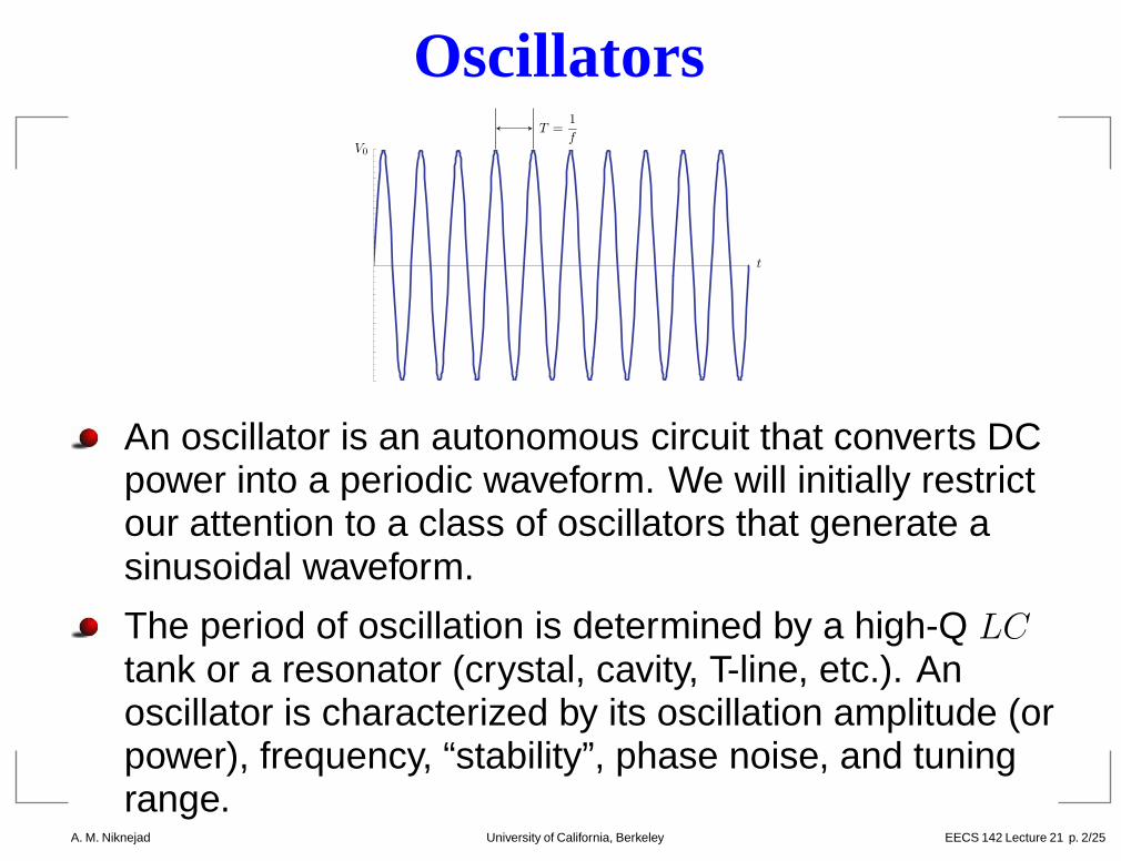
An oscillator is an autonomous circuit that converts DCpower into a periodic waveform. We will initially restrictour attention to a class of oscillators that generate asinusoidal waveform.
The period of oscillation is determined by a high-Q LCtank or a resonator (crystal, cavity, T-line, etc.). Anoscillator is characterized by its oscillation amplitude (orpower), frequency, “stability”, phase noise, and tuningrange.
A. M. Niknejad University of California, Berkeley EECS 142 Lecture 21 p. 2/25 – p. 2/25
Oscillators (cont)Disturbance
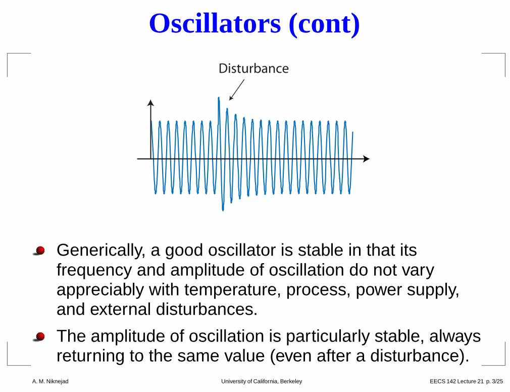
Generically, a good oscillator is stable in that itsfrequency and amplitude of oscillation do not varyappreciably with temperature, process, power supply,and external disturbances.
The amplitude of oscillation is particularly stable, alwaysreturning to the same value (even after a disturbance).
A. M. Niknejad University of California, Berkeley EECS 142 Lecture 21 p. 3/25 – p. 3/25
Phase Noise
ω0
Phase Noise
ω0 + δω
L(δω) ∼ 100 dB
LC Tank Alone
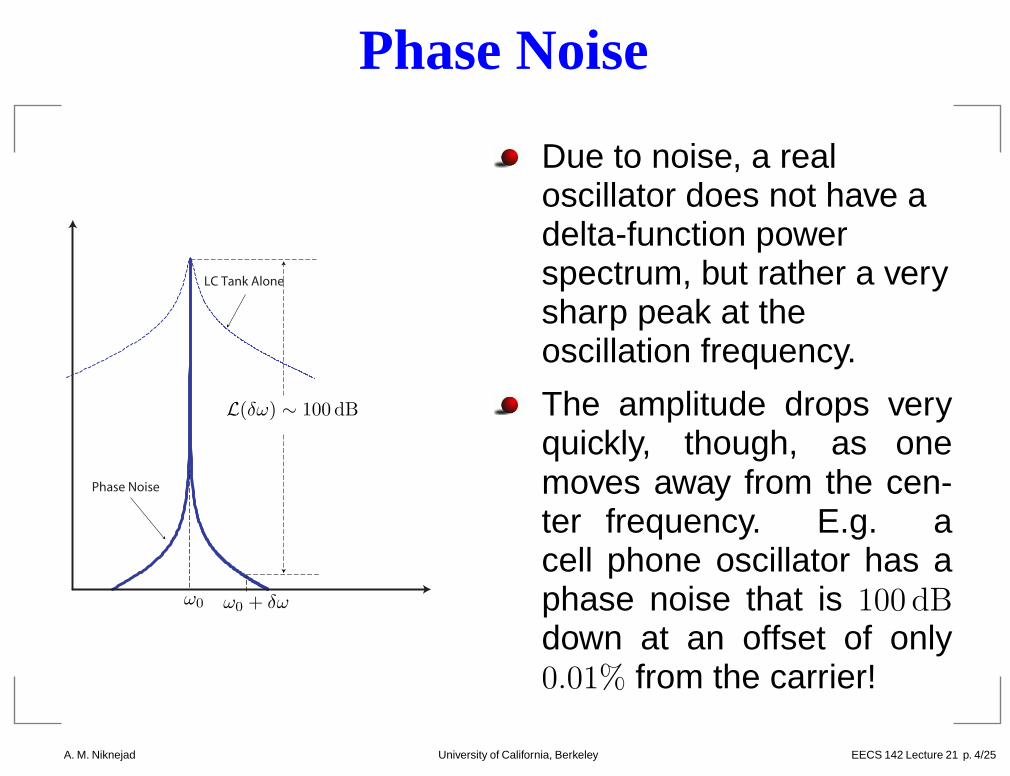
Due to noise, a realoscillator does not have adelta-function powerspectrum, but rather a verysharp peak at theoscillation frequency.
The amplitude drops veryquickly, though, as onemoves away from the cen-ter frequency. E.g. acell phone oscillator has aphase noise that is 100 dBdown at an offset of only0.01% from the carrier!
A. M. Niknejad University of California, Berkeley EECS 142 Lecture 21 p. 4/25 – p. 4/25
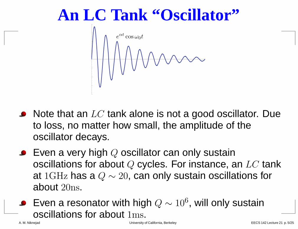
An LC Tank “Oscillator”eαt cos ω0t
Note that an LC tank alone is not a good oscillator. Dueto loss, no matter how small, the amplitude of theoscillator decays.
Even a very high Q oscillator can only sustainoscillations for about Q cycles. For instance, an LC tankat 1GHz has a Q 20, can only sustain oscillations forabout 20ns.
Even a resonator with high Q 106, will only sustainoscillations for about 1ms.
A. M. Niknejad University of California, Berkeley EECS 142 Lecture 21 p. 5/25 – p. 5/25
Feedback Perspective
vo
−vo
n
gmvin : 1
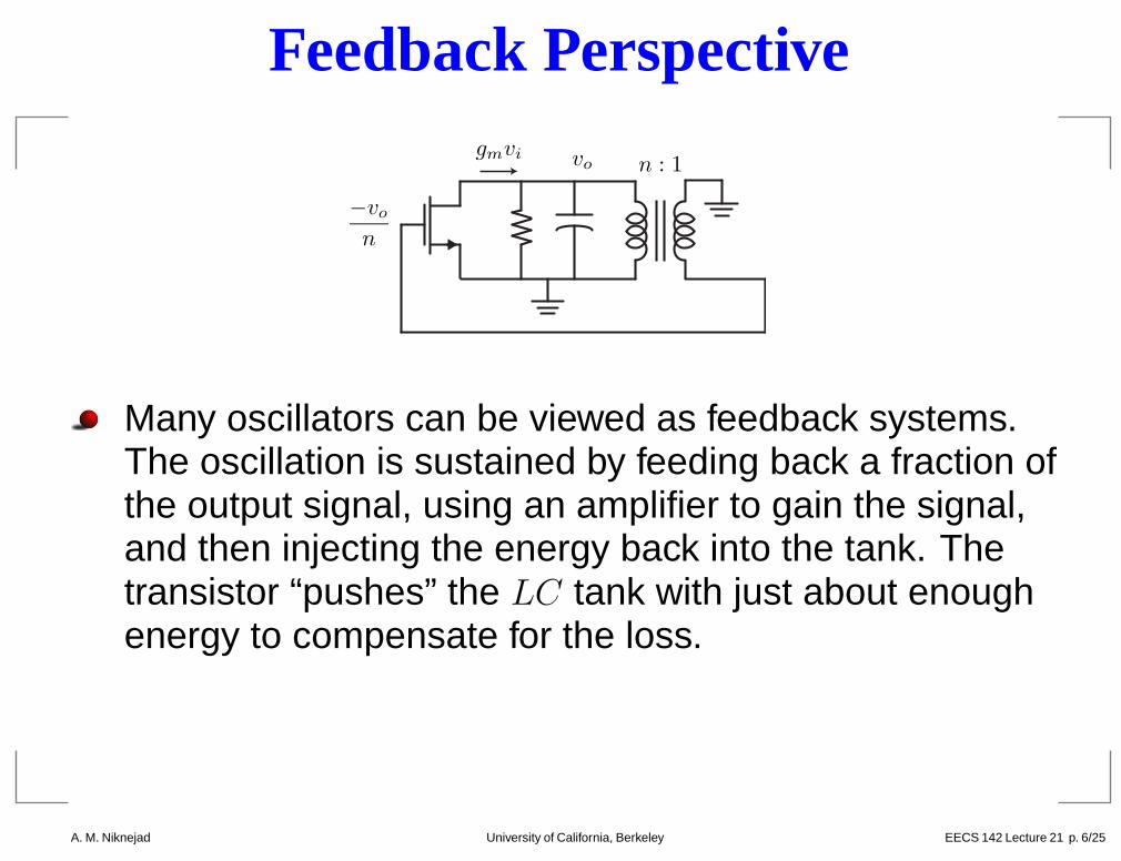
Many oscillators can be viewed as feedback systems.The oscillation is sustained by feeding back a fraction ofthe output signal, using an amplifier to gain the signal,and then injecting the energy back into the tank. Thetransistor “pushes” the LC tank with just about enoughenergy to compensate for the loss.
A. M. Niknejad University of California, Berkeley EECS 142 Lecture 21 p. 6/25 – p. 6/25
Negative Resistance Perspective
Active
Circuit
Negative
Resistance
LC Tank
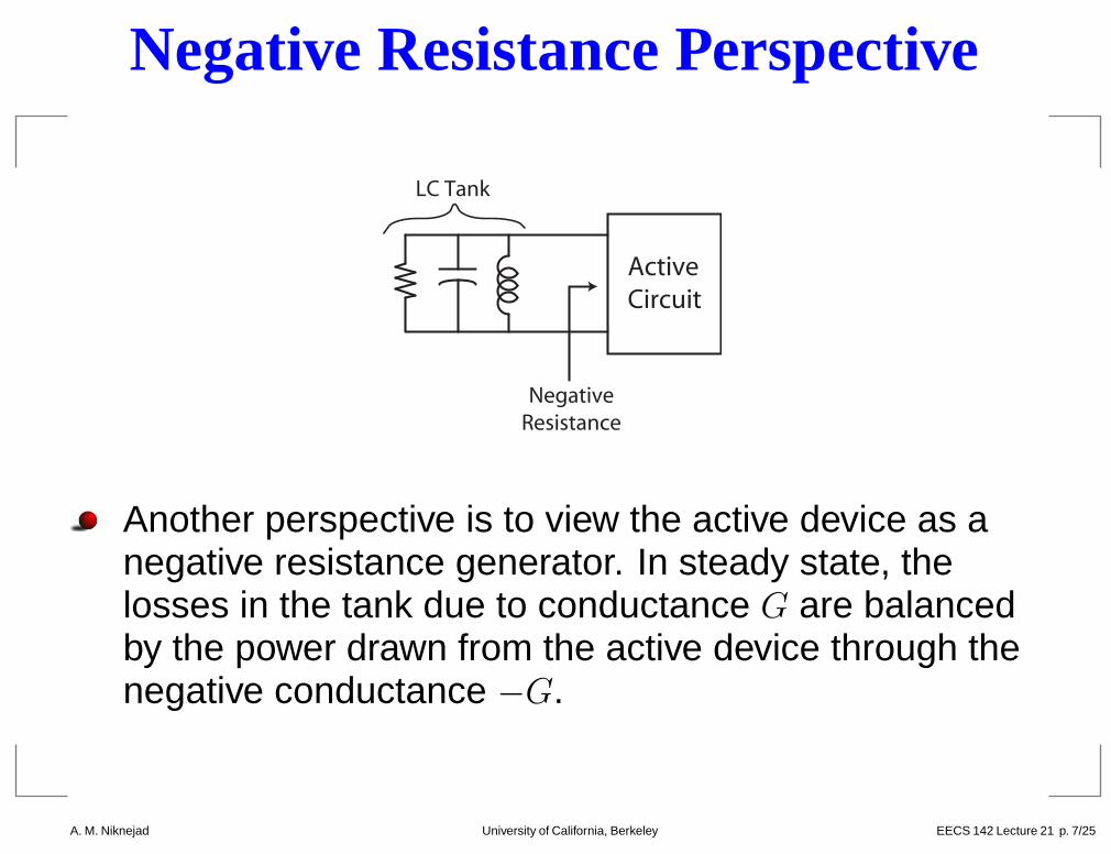
Another perspective is to view the active device as anegative resistance generator. In steady state, thelosses in the tank due to conductance G are balancedby the power drawn from the active device through thenegative conductance G.
A. M. Niknejad University of California, Berkeley EECS 142 Lecture 21 p. 7/25 – p. 7/25
Feedback Approach
si(s) so(s)+
−a(s)
f(s)
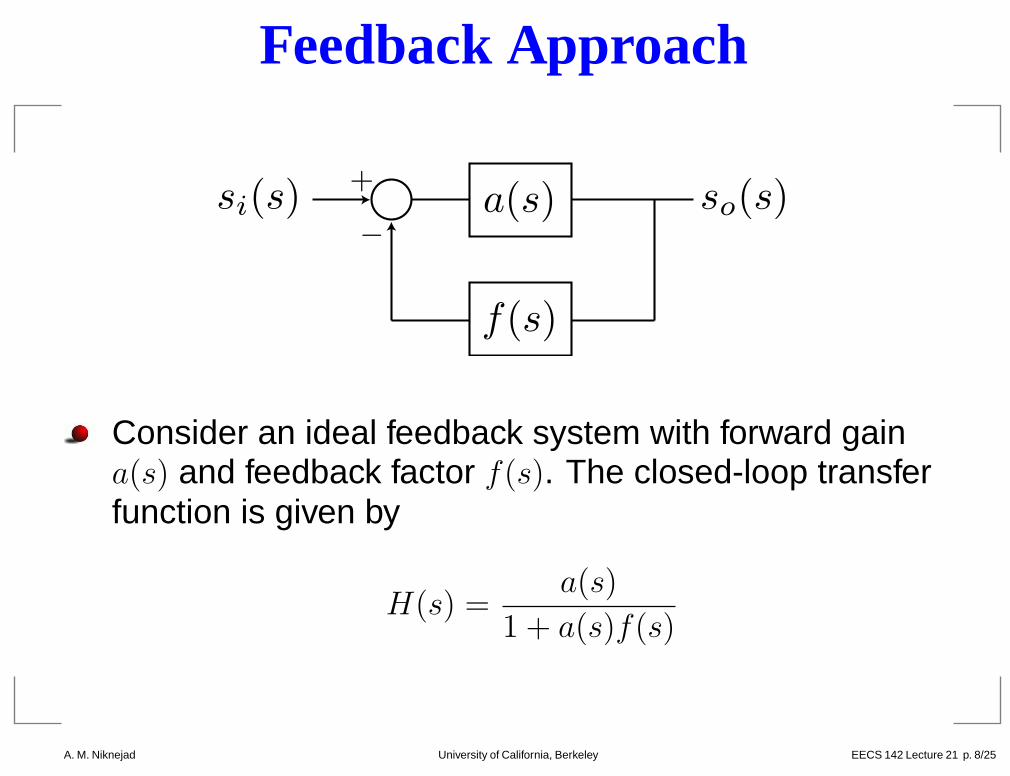
Consider an ideal feedback system with forward gaina(s) and feedback factor f(s). The closed-loop transferfunction is given by
H(s) =a(s)
1 + a(s)f(s)
A. M. Niknejad University of California, Berkeley EECS 142 Lecture 21 p. 8/25 – p. 8/25
Feedback Example
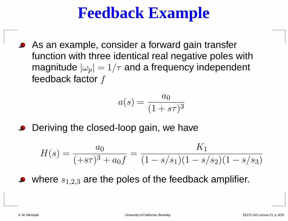
As an example, consider a forward gain transferfunction with three identical real negative poles withmagnitude |ωp| = 1/τ and a frequency independentfeedback factor f
a(s) =a0
(1 + sτ)3
Deriving the closed-loop gain, we have
H(s) =a0
(+sτ)3 + a0f=
K1
(1 s/s1)(1 s/s2)(1 s/s3)
where s1,2,3 are the poles of the feedback amplifier.
A. M. Niknejad University of California, Berkeley EECS 142 Lecture 21 p. 9/25 – p. 9/25
Poles of Closed-Loop Gain
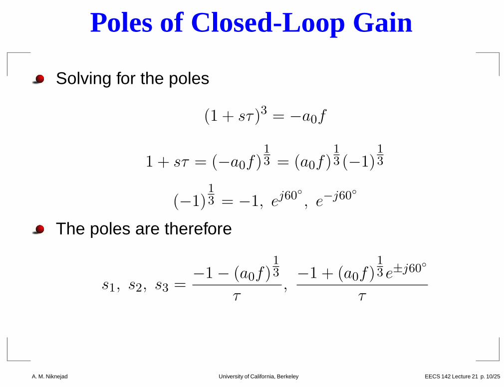
Solving for the poles
(1 + sτ)3 = a0f
1 + sτ = ( a0f)1
3 = (a0f)1
3 ( 1)1
3
( 1)1
3 = 1, ej60◦
, e−j60◦
The poles are therefore
s1, s2, s3 =1 (a0f)
1
3
τ,
1 + (a0f)1
3 e±j60◦
τ
A. M. Niknejad University of California, Berkeley EECS 142 Lecture 21 p. 10/25 – p
Root Locus
jω
σ+60◦
−60◦
−1
τ
a0f = 0
a0f = 8
j√
3/τ
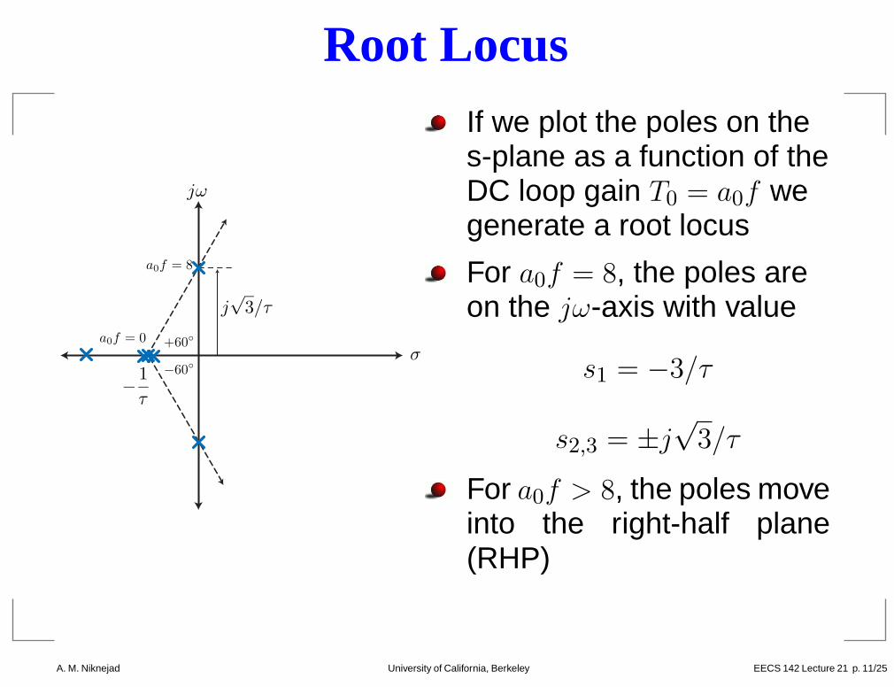
If we plot the poles on thes-plane as a function of theDC loop gain T0 = a0f wegenerate a root locus
For a0f = 8, the poles areon the jω-axis with value
s1 = 3/τ
s2,3 = ±j√
3/τ
For a0f > 8, the poles moveinto the right-half plane(RHP)
A. M. Niknejad University of California, Berkeley EECS 142 Lecture 21 p. 11/25 – p
Natural Response
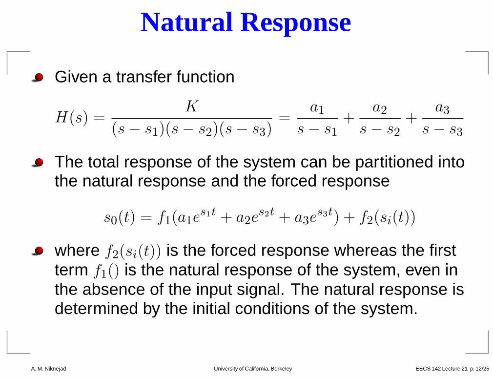
Given a transfer function
H(s) =K
(s − s1)(s − s2)(s − s3)=
a1
s − s1
+a2
s − s2
+a3
s − s3
The total response of the system can be partitioned intothe natural response and the forced response
s0(t) = f1(a1es1t + a2e
s2t + a3es3t) + f2(si(t))
where f2(si(t)) is the forced response whereas the firstterm f1() is the natural response of the system, even inthe absence of the input signal. The natural response isdetermined by the initial conditions of the system.
A. M. Niknejad University of California, Berkeley EECS 142 Lecture 21 p. 12/25 – p
Real LHP Poles
e−αt
Stable systems have all poles in the left-half plane(LHP).
Consider the natural response when the pole is on thenegative real axis, such as s1 for our examples.
The response is a decaying exponential that dies awaywith a time-constant determined by the pole magnitude.
A. M. Niknejad University of California, Berkeley EECS 142 Lecture 21 p. 13/25 – p
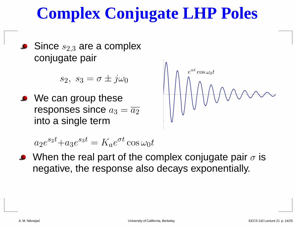
Complex Conjugate LHP Poles
Since s2,3 are a complexconjugate pair
s2, s3 = σ ± jω0
We can group theseresponses since a3 = a2
into a single term
a2es2t+a3e
s3t = Kaeσt cos ω0t
eαt cos ω0t
When the real part of the complex conjugate pair σ isnegative, the response also decays exponentially.
A. M. Niknejad University of California, Berkeley EECS 142 Lecture 21 p. 14/25 – p
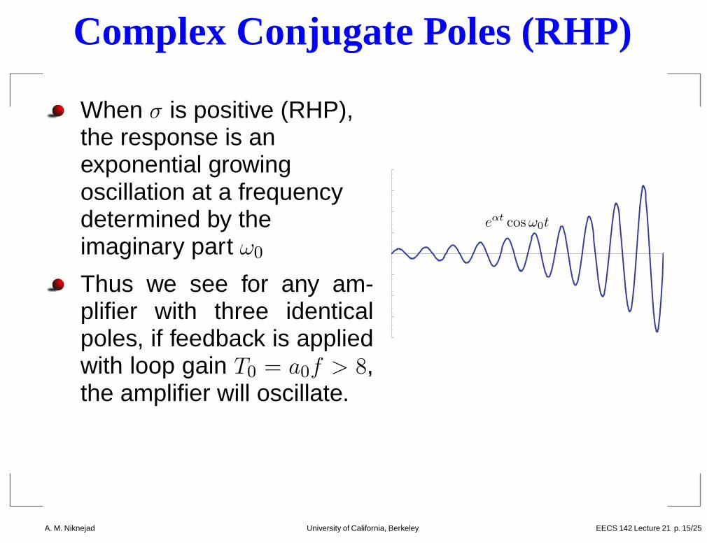
Complex Conjugate Poles (RHP)
When σ is positive (RHP),the response is anexponential growingoscillation at a frequencydetermined by theimaginary part ω0
Thus we see for any am-plifier with three identicalpoles, if feedback is appliedwith loop gain T0 = a0f > 8,the amplifier will oscillate.
αte cos ω0t
A. M. Niknejad University of California, Berkeley EECS 142 Lecture 21 p. 15/25 – p
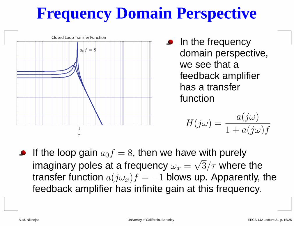
Frequency Domain Perspective
1
τ
a0f = 8
Closed Loop Transfer Function
In the frequencydomain perspective,we see that afeedback amplifierhas a transferfunction
H(jω) =a(jω)
1 + a(jω)f
If the loop gain a0f = 8, then we have with purelyimaginary poles at a frequency ωx =
√3/τ where the
transfer function a(jωx)f = −1 blows up. Apparently, thefeedback amplifier has infinite gain at this frequency.
A. M. Niknejad University of California, Berkeley EECS 142 Lecture 21 p. 16/25 – p
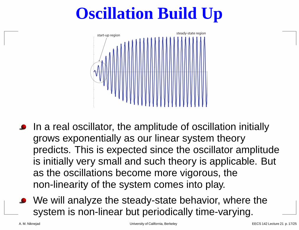
Oscillation Build Upstart-up region
steady-state region
In a real oscillator, the amplitude of oscillation initiallygrows exponentially as our linear system theorypredicts. This is expected since the oscillator amplitudeis initially very small and such theory is applicable. Butas the oscillations become more vigorous, thenon-linearity of the system comes into play.
We will analyze the steady-state behavior, where thesystem is non-linear but periodically time-varying.
A. M. Niknejad University of California, Berkeley EECS 142 Lecture 21 p. 17/25 – p
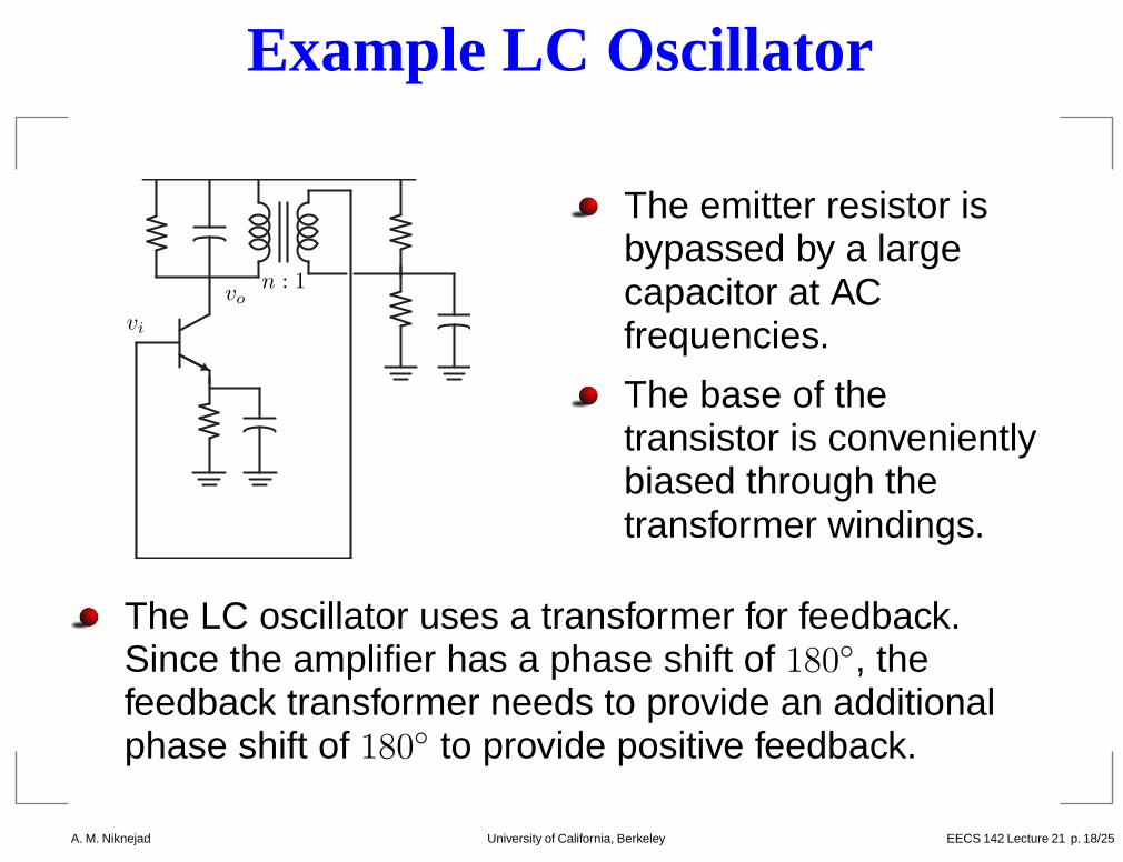
Example LC Oscillator
vo
vi
n : 1
The emitter resistor isbypassed by a largecapacitor at ACfrequencies.
The base of thetransistor is convenientlybiased through thetransformer windings.
The LC oscillator uses a transformer for feedback.Since the amplifier has a phase shift of 180◦, thefeedback transformer needs to provide an additionalphase shift of 180◦ to provide positive feedback.
A. M. Niknejad University of California, Berkeley EECS 142 Lecture 21 p. 18/25 – p
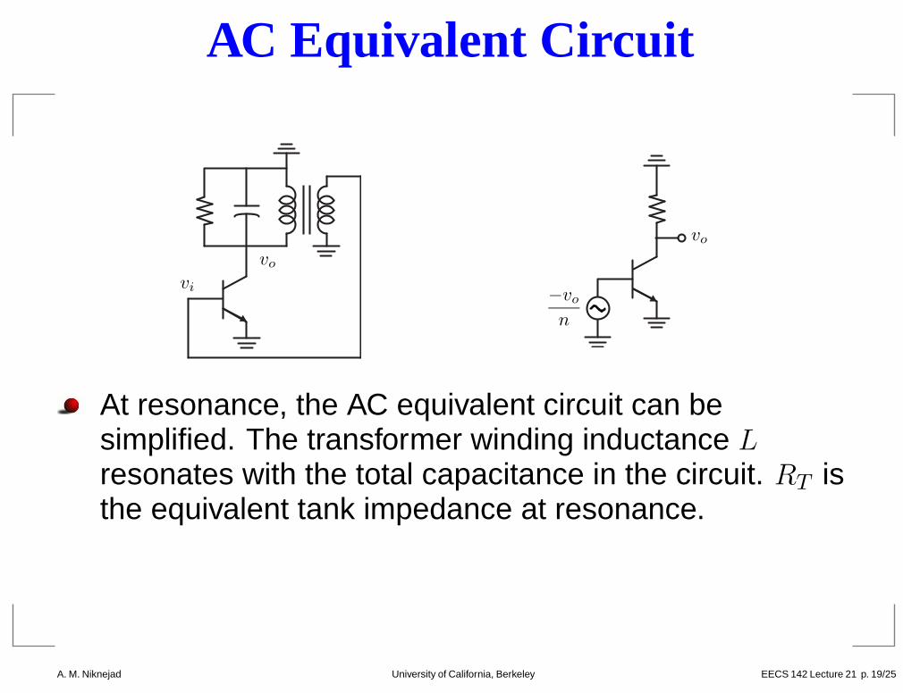
AC Equivalent Circuit
vo
vi
vo
−vo
n
At resonance, the AC equivalent circuit can besimplified. The transformer winding inductance Lresonates with the total capacitance in the circuit. RT isthe equivalent tank impedance at resonance.
A. M. Niknejad University of California, Berkeley EECS 142 Lecture 21 p. 19/25 – p
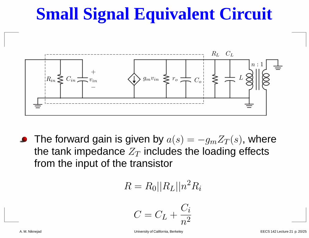
Small Signal Equivalent Circuit
roCingmvin
+vin
−Rin Co
CLRL
L
n : 1
The forward gain is given by a(s) = −gmZT (s), wherethe tank impedance ZT includes the loading effectsfrom the input of the transistor
R = R0||RL||n2Ri
C = CL +Ci
n2
A. M. Niknejad University of California, Berkeley EECS 142 Lecture 21 p. 20/25 – p
Open-Loop Transfer Function
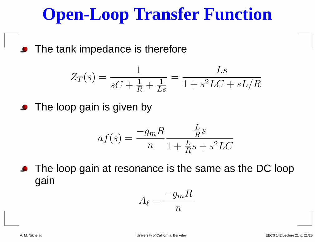
The tank impedance is therefore
ZT (s) =1
sC + 1
R+ 1
Ls
=Ls
1 + s2LC + sL/R
The loop gain is given by
af(s) =−gmR
n
LR
s
1 + LR
s + s2LC
The loop gain at resonance is the same as the DC loopgain
Aℓ =−gmR
n
A. M. Niknejad University of California, Berkeley EECS 142 Lecture 21 p. 21/25 – p
Closed-Loop Transfer Function
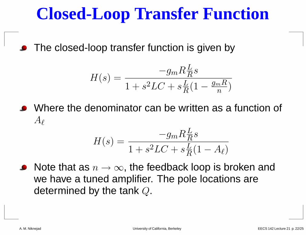
The closed-loop transfer function is given by
H(s) =−gmRL
Rs
1 + s2LC + sLR
(1 − gmRn
)
Where the denominator can be written as a function ofAℓ
H(s) =−gmRL
Rs
1 + s2LC + sLR
(1 − Aℓ)
Note that as n → ∞, the feedback loop is broken andwe have a tuned amplifier. The pole locations aredetermined by the tank Q.
A. M. Niknejad University of California, Berkeley EECS 142 Lecture 21 p. 22/25 – p
Oscillator Closed-Loop Gain vsAℓ
Aℓ < 1
Aℓ = 1
ω0 =
√
1
LC
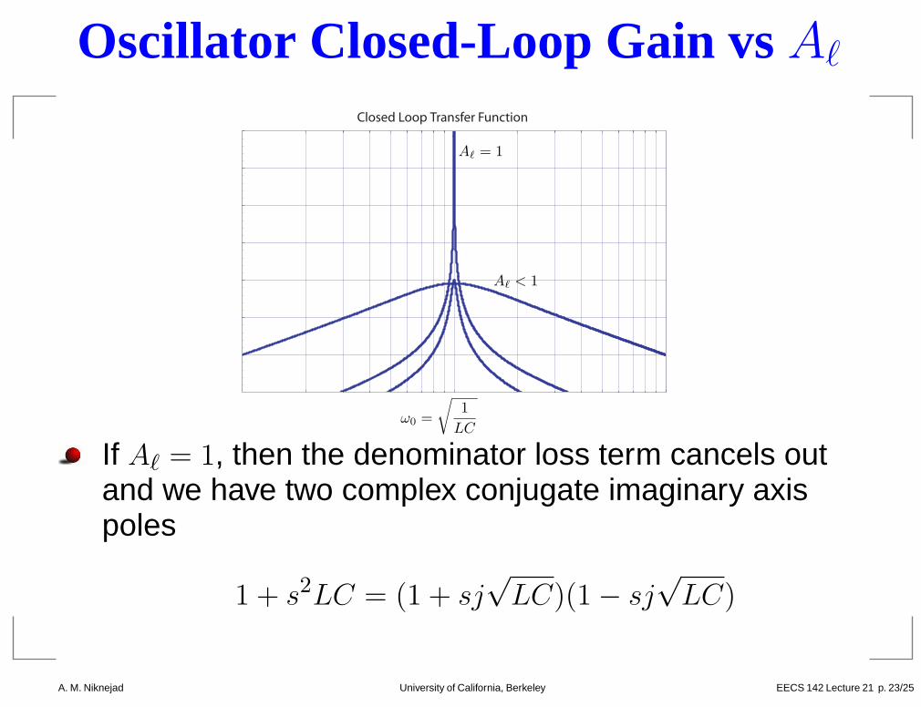
Closed Loop Transfer Function
If Aℓ = 1, then the denominator loss term cancels outand we have two complex conjugate imaginary axispoles
1 + s2LC = (1 + sj√
LC)(1 − sj√
LC)
A. M. Niknejad University of California, Berkeley EECS 142 Lecture 21 p. 23/25 – p
Root Locus for LC Oscillator
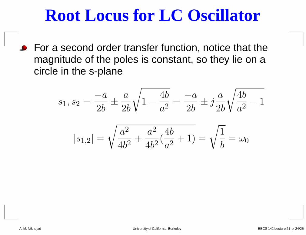
For a second order transfer function, notice that themagnitude of the poles is constant, so they lie on acircle in the s-plane
s1, s2 =−a
2b± a
2b
√
1 − 4b
a2=
−a
2b± j
a
2b
√
4b
a2− 1
|s1,2| =
√
a2
4b2+
a2
4b2(4b
a2+ 1) =
√
1
b= ω0
A. M. Niknejad University of California, Berkeley EECS 142 Lecture 21 p. 24/25 – p
Root Locus (cont)
"""""""""
"
""""""""""
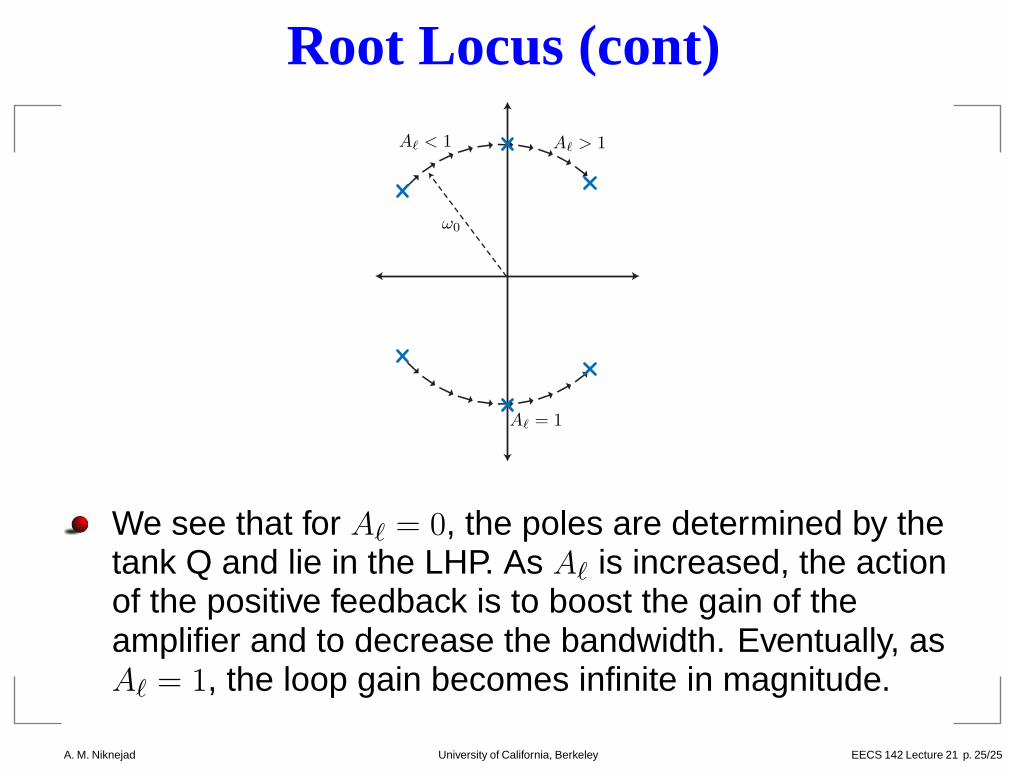
ω0
Aℓ < 1 Aℓ > 1
Aℓ = 1
We see that for Aℓ = 0, the poles are determined by thetank Q and lie in the LHP. As Aℓ is increased, the actionof the positive feedback is to boost the gain of theamplifier and to decrease the bandwidth. Eventually, asAℓ = 1, the loop gain becomes infinite in magnitude.
A. M. Niknejad University of California, Berkeley EECS 142 Lecture 21 p. 25/25 – p