22-1

Lecture 22

Multiple Comparisons

STAT 512

Spring 2011

Background Reading

KNNL: 17.1-17.3

22-2

Topic Overview

• Estimating Factor Level Means

• Standard Errors for Means

• Pairwise Comparisons

22-3

Analysis of Factor Level Means

• F-test is significant; there exist differences among the means. Now what?

• Want to determine which means are

different. Form groups of means that are

statistically the same.

22-4

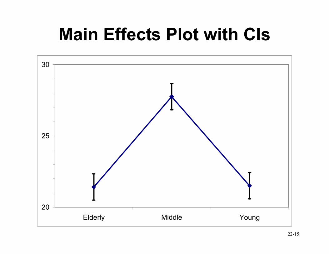
Visual Assessment

• Can often get an idea by looking at plots

� Side-by-side Box Plots

� Plots of the factor level means (called

Main Effects Plots)

� Bar Graphs

• These plots do not give any information

about the precision of the estimates. Need

to consider standard errors.

22-5

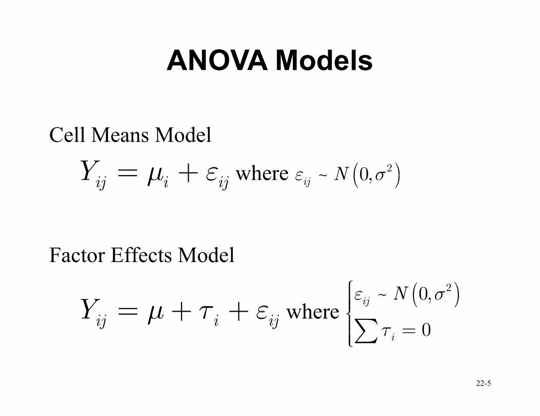
ANOVA Models

Cell Means Model

ij i ijY µ ε= + where ( )2~ 0,ij Nε σ

Factor Effects Model

ij i ijY µ τ ε= + + where ( )2~ 0,

0

ij

i

Nε σ

τ

=∑

22-6

Estimates

• Overall or grand mean is

1

ij

i j

Y YN

= ∑∑ii

• Mean for factor level i is

1

i i ij

ji

Y Yn

µ = = ∑i

• Factor Effects estimated by

i iY Yτ = −i ii

(note N=nT)

22-7

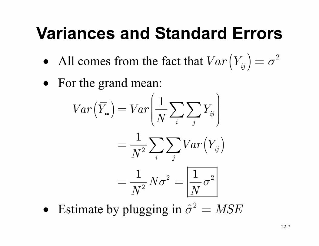
Variances and Standard Errors

• All comes from the fact that ( ) 2ijVar Y σ=

• For the grand mean:

( )

( )2

2 2

2

1

1

1 1

ij

i j

ij

i j

Var Y Var YN

Var YN

NN N

σ σ

=

=

= =

∑∑

∑∑

ii

• Estimate by plugging in 2ˆ MSEσ =

22-8

Cell Mean Variances

• For cell means (fixed level i):

( )

( )2

2 2

2

1

1

1 1

i ij

ji

ij

ji

i

i i

Var Y Var Yn

Var Yn

nn nσ σ

=

=

= =

∑

∑

i

• Again plug in 2ˆ MSEσ = to get the

estimate.

22-9

Standard Error of the Mean

• � ( ) /SE Y MSE N=ii

• � ( ) /i iSE Y MSE n=i

• Used to develop confidence intervals

22-10

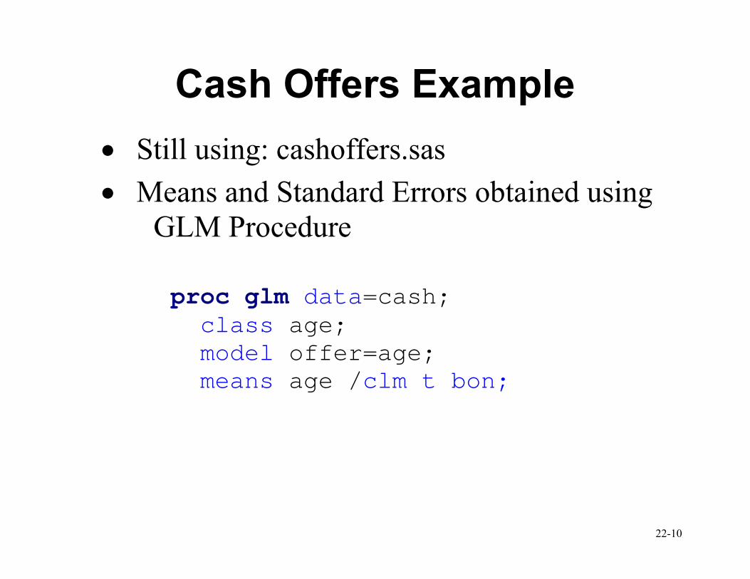
Cash Offers Example

• Still using: cashoffers.sas

• Means and Standard Errors obtained using

GLM Procedure

proc glm data=cash; class age; model offer=age; means age /clm t bon;

22-11

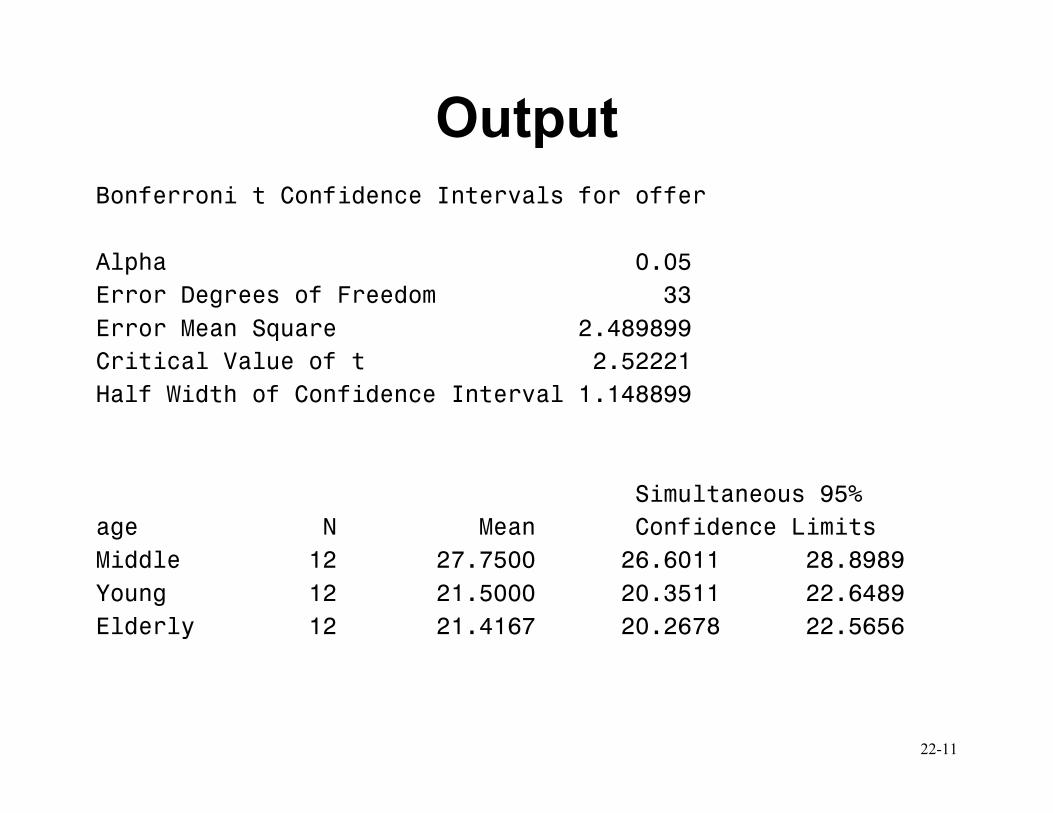
Output

Bonferroni t Confidence Intervals for offer

Alpha 0.05

Error Degrees of Freedom 33

Error Mean Square 2.489899

Critical Value of t 2.52221

Half Width of Confidence Interval 1.148899

Simultaneous 95%

age N Mean Confidence Limits

Middle 12 27.7500 26.6011 28.8989

Young 12 21.5000 20.3511 22.6489

Elderly 12 21.4167 20.2678 22.5656

22-12

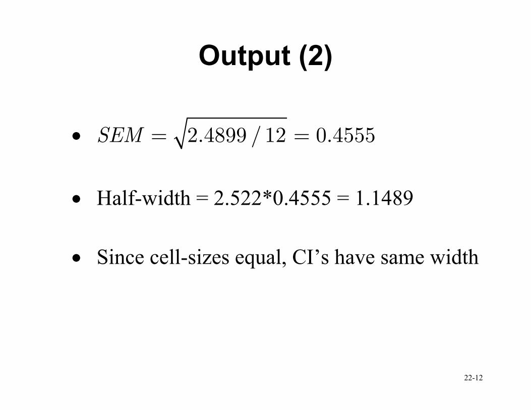
Output (2)

• 2.4899 / 12 0.4555SEM = =

• Half-width = 2.522*0.4555 = 1.1489

• Since cell-sizes equal, CI’s have same width

22-13

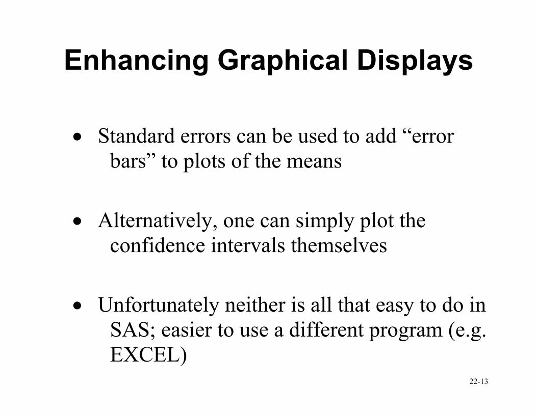
Enhancing Graphical Displays

• Standard errors can be used to add “error bars” to plots of the means

• Alternatively, one can simply plot the

confidence intervals themselves

• Unfortunately neither is all that easy to do in SAS; easier to use a different program (e.g.

EXCEL)

22-14

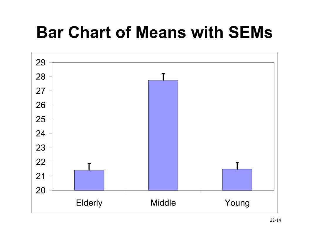
Bar Chart of Means with SEMs

20

21

22

23

24

25

26

27

28

29

Elderly Middle Young

22-15

Main Effects Plot with CIs

20

25

30

Elderly Middle Young

22-16

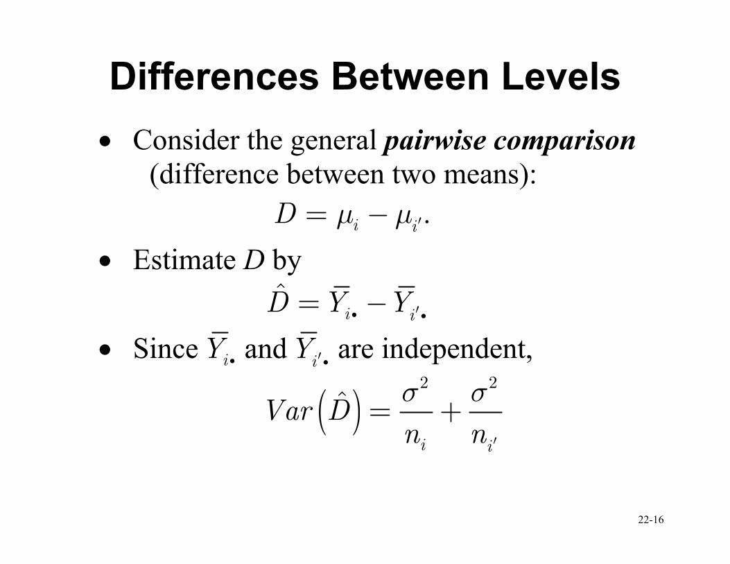
Differences Between Levels

• Consider the general pairwise comparison (difference between two means):

i iD µ µ ′= − .

• Estimate D by

ˆi i

D Y Y ′= −i i

• Since iY i and iY ′i are independent,

( )2 2

ˆ

i i

Var Dn n

σ σ

′

= +

22-17

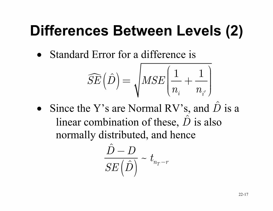
Differences Between Levels (2)

• Standard Error for a difference is

� ( ) 1 1ˆ

i i

SE D MSEn n ′

= +

• Since the Y’s are Normal RV’s, and D is a

linear combination of these, D is also

normally distributed, and hence

( )ˆ

~ˆ Tn r

D Dt

SE D−

−

22-18

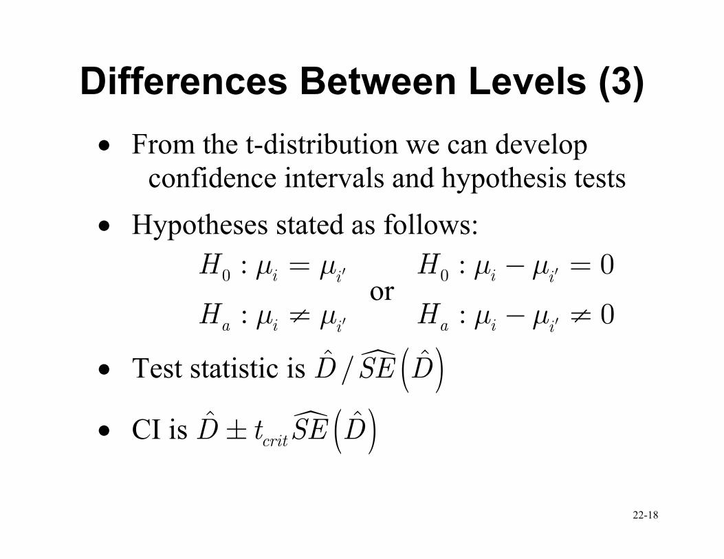
Differences Between Levels (3)

• From the t-distribution we can develop

confidence intervals and hypothesis tests

• Hypotheses stated as follows:

0 :

:

i i

a i i

H

H

µ µ

µ µ

′

′

=

≠ or

0 : 0

: 0

i i

a i i

H

H

µ µ

µ µ

′

′

− =

− ≠

• Test statistic is � ( )ˆ ˆ/D SE D

• CI is � ( )ˆ ˆcritD t SE D±

22-19

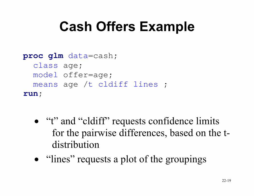
Cash Offers Example

proc glm data=cash; class age; model offer=age; means age /t cldiff lines ; run;

• “t” and “cldiff” requests confidence limits

for the pairwise differences, based on the t-

distribution

• “lines” requests a plot of the groupings

22-20

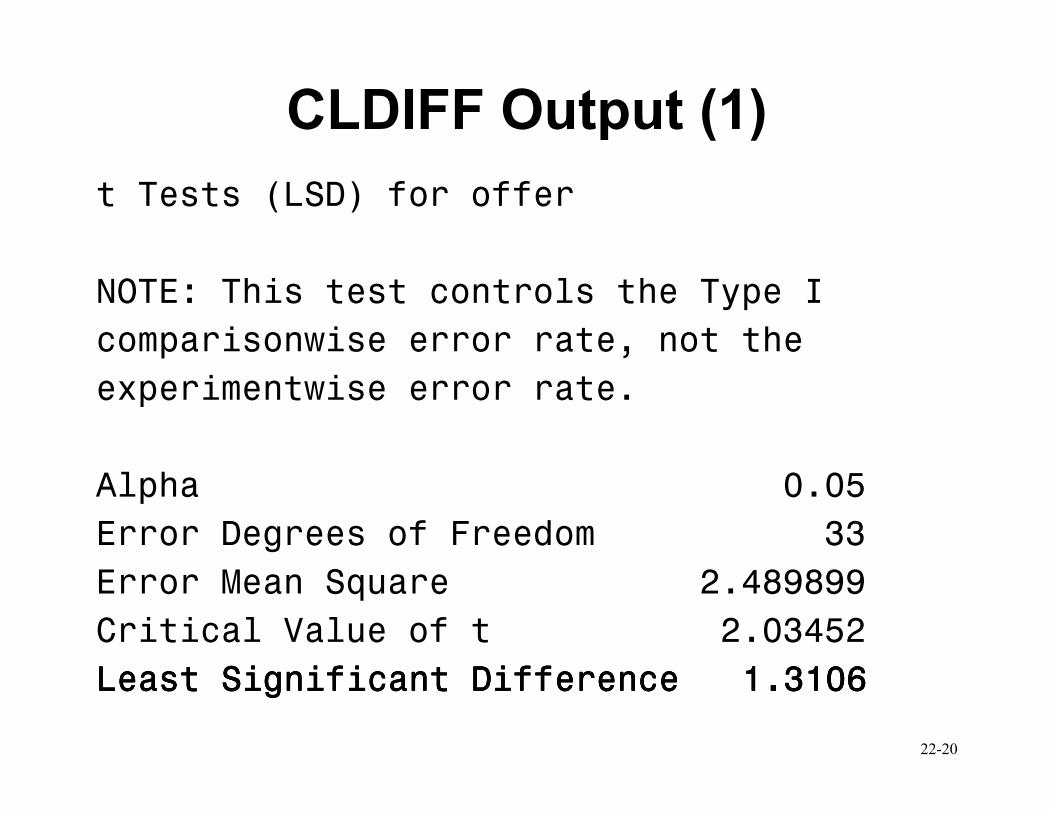
CLDIFF Output (1)

t Tests (LSD) for offer

NOTE: This test controls the Type I

comparisonwise error rate, not the

experimentwise error rate.

Alpha 0.05

Error Degrees of Freedom 33

Error Mean Square 2.489899

Critical Value of t 2.03452

Least Significant Difference 1.3106Least Significant Difference 1.3106Least Significant Difference 1.3106Least Significant Difference 1.3106

22-21

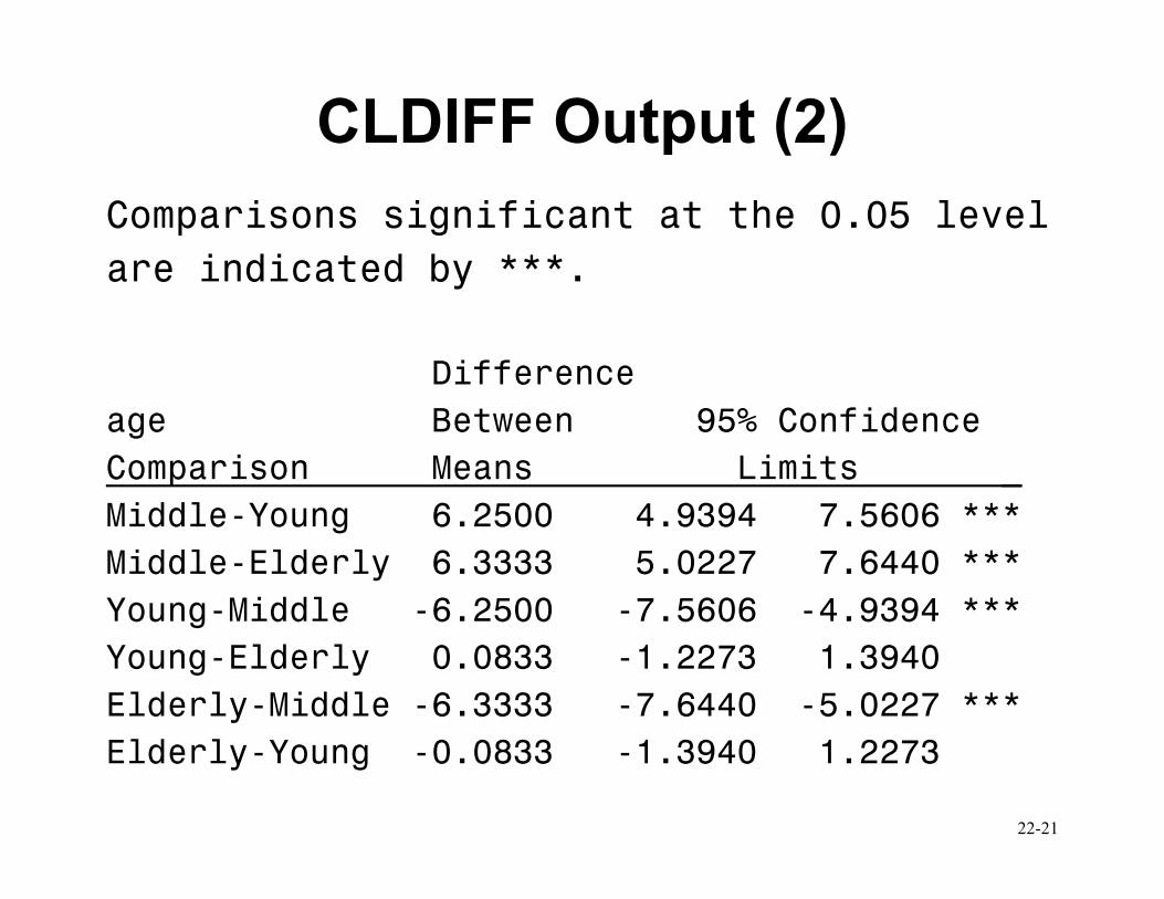
CLDIFF Output (2)

Comparisons significant at the 0.05 level

are indicated by ***.

Difference

age Between 95% Confidence

Comparison Means Limits _

Middle-Young 6.2500 4.9394 7.5606 ***

Middle-Elderly 6.3333 5.0227 7.6440 ***

Young-Middle -6.2500 -7.5606 -4.9394 ***

Young-Elderly 0.0833 -1.2273 1.3940

Elderly-Middle -6.3333 -7.6440 -5.0227 ***

Elderly-Young -0.0833 -1.3940 1.2273

22-22

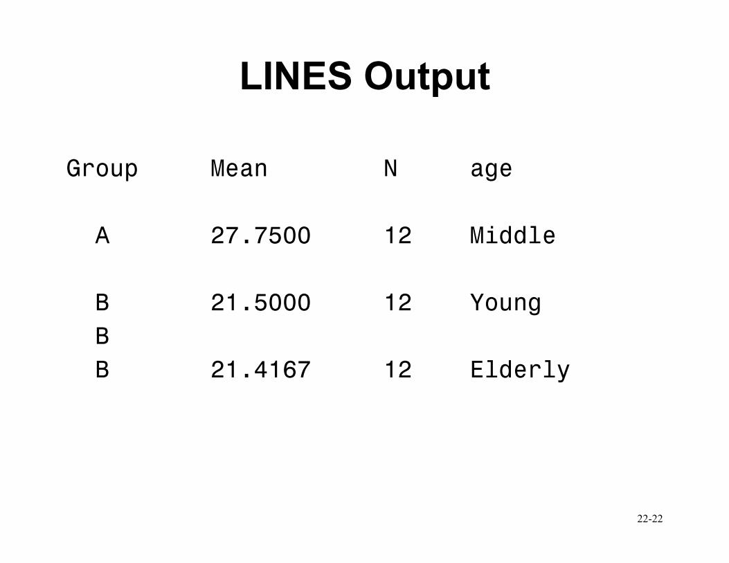
LINES Output

Group Mean N age

A 27.7500 12 Middle

B 21.5000 12 Young

B

B 21.4167 12 Elderly

22-23

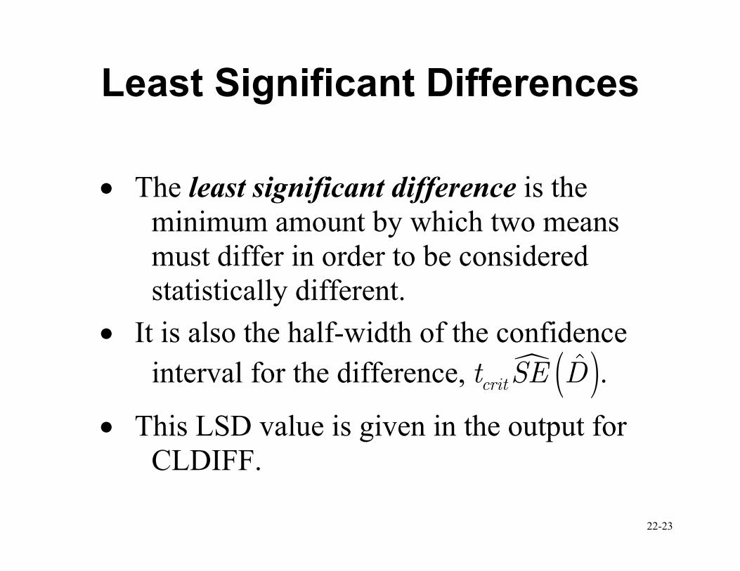
Least Significant Differences

• The least significant difference is the minimum amount by which two means

must differ in order to be considered

statistically different.

• It is also the half-width of the confidence

interval for the difference, � ( )ˆcritt SE D .

• This LSD value is given in the output for CLDIFF.

22-24

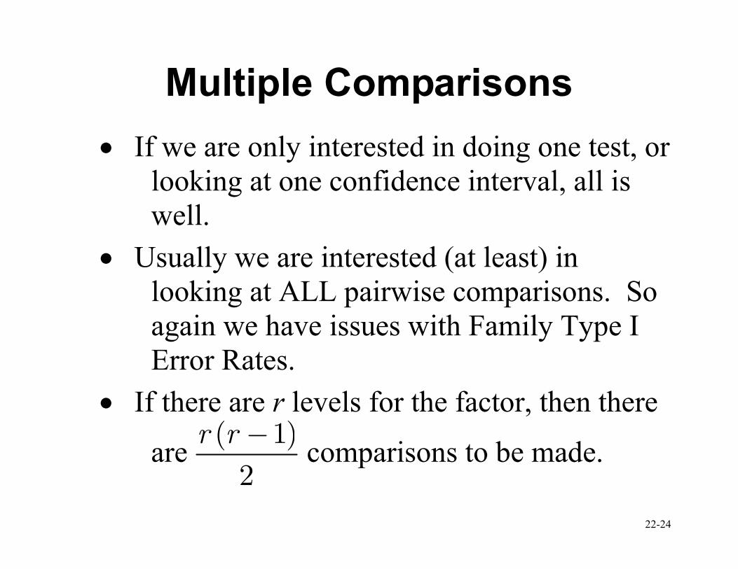
Multiple Comparisons

• If we are only interested in doing one test, or looking at one confidence interval, all is

well.

• Usually we are interested (at least) in looking at ALL pairwise comparisons. So

again we have issues with Family Type I

Error Rates.

• If there are r levels for the factor, then there

are ( )1

2

r r − comparisons to be made.

22-25

Bonferroni

• A Bonferroni adjustment works OK when r

is small (2, 3, or 4).

• For r > 4, Bonferroni starts to get much

more conservative than necessary

• Alternative multiple comparison procedures

have been developed.

22-26

Preview: Other Methods

• Simple pair-wise comparisons can be

accomplished all at once using Tukey

adjustments.

• If we are just interested in comparing

treatments to a control, Dunnett’s test is

slightly superior to Tukey.

• If we are searching through the data for something significant (data snooping),

then Scheffe provides more conservative

critical values.

22-27

Upcoming in Lecture 23...

• Linear Combinations & Contrasts

• More on Multiple Comparisons