2017/10/10

1

Lecture 2b: International flow of tourism

Prof. Andrea Saayman – NWU

Demand Theory The demand curve, indifference curves and budget

constraints Price changes

Income and substitution effects

Marshallian versus Hicksian demand curves Price elasticities Income elasticities

Tourism demand AIDS framework Calculating elasticities

Case studies

Key Points

2017/10/10

2

Illustrate and explain the influence of a change in the price on the demand for a product, referring to both income and substitution effects

Distinguish between a Marshallian and Hicksian demand function

Distinguish between and be able to calculate and interpret various price elasticities and income elasticity

Identify complementary and substitute goods Explain the difference between necessities, inferior and

luxury goods Provide a framework for determining the elasticities of a

destination Interpret case study results from an Almost Ideal Demand

System

Outcomes

Generally we specify demand as: x1 = f(p1, p2, m)

x2 = f(p2, p1, m)

with consumers wanting to maximiseutility: max U(x1,x2)

Given their budget constraints: m=p1x1+p2x2

Optimal choice is where slope of indifference curve (MRS) equals slope of budget line (-p1/p2)

Demand Theory

2017/10/10

3

Demand TheoryDemand curves

• Show relationship between quantity demanded and price of a product

– Downward-sloping

– A, B and C = different possible combinations

– Different elasticities

• Position depend on income

– Increase in income = shift to right

– Decrease in income = shift to left

Price

Quantity

Demand

A

B

C

PA

QA

PB

PC

QB QC

Demand TheoryIndifference curves• Properties of consumer

preferences:– Completeness– Transitivity– More is better

• Indifference curve– Set of bundles of goods which are

equally desirable– Complete set of indifference

curves = preference map• Further away from origin are

preferred• There is an IC through every

possible bundle• Cannot cross• Slope downwards

– Willingness to substitute between goods = MRS = slope of the IC.

Good

x2

Good x1

IC 3

IC 2

IC1

2017/10/10

4

Demand TheoryTypes of indifference curves

• Perfect substitutes • Perfect complements

Good x

2

Good x1G

ood x

2Good x1

IC 2IC 1

IC 2

IC 1

Demand TheoryBudget Constraint

• Most important constraint to preferences

• Allocate budget/income between 2 goods

• Budget line = visual presentation of budget constraint

– Trade-off market imposes on how much of good x2 must be given up to get 1 extra of good x1 =

MRT = slope of the budget line

Good x

2

Good x1

m/p2

m/p1

BL

2017/10/10

5

Demand TheoryBudget Constraint

• Change in income • Change in price

Good x

2Good x1

Good x

2

Good x1

BL 2BL 1 BL 2BL 1

Optimal demand

x2

x1

x2*

x1*

IC3

IC2

IC1

BL

a

2017/10/10

6

Change in price

x1*

c

x1**

x2**

b

x2

x1

x2*

IC3

IC2

BL1

a

BL2

Suppose p1 increases

Demand for x1 will decrease

Two effects present:

Substitution effect – change in demand due to change in rate of exchange between x1

and x2 (a to b)

Income effect – change in demand due to having less purchasing power (b to c)

Change in price

2017/10/10

7

Change in priceTwo demand curves

Marhallian demand

• By Alfred Marshall

• Origin in utility maximization

• Relates price (p) and income (m) to bundle (x) demanded

• Observable demand function

• Combine income and substitution effects

Hicksian demand

)(max),( xumpv

• By J.R. Hicks

• Origin in expenditure (or cost) function

• Shows minimum expenditure needed to achieve a certain level of utility at prices (p)

• Demand when U is kept constant while p changes

• Not a directly observable demand function

• Only substitution effects

pxupe min*),(

Change in priceTwo demand curves

• Hicksian demand curve (xc)

– Steeper

– Only substitution effect

• Marshallian demand curve (x)

– Flatter

– Both income and substitution effect

2017/10/10

8

Elasticity measures the impact a small (1%) change in price (or other factors) on the quantity demanded.

Types:

Own-price elasticity = and

Cross-price elasticity = and

Income elasticity = and

Price elasticities

1

1

%

%

p

x

2

2

%

%

p

x

1

2

%

%

p

x

2

1

%

%

p

x

m

x

%

% 1

m

x

%

% 2

Own Price Elasticity

0-1

Perfectly

Elastic

Relatively InelasticRelatively Elastic

UNITARY Elastic

Perfectly Inelastic

2017/10/10

9

Own Price Elasticity –what does it look like?

p

x

p

x

p

x

p

x

p

x

e=?

e=?

e=?e=?

e=?

Price elasticities

How to calculate the

elasticity from the graph:

• 𝑒 =∆𝑥

∆𝑝×

𝑝

𝑥=

1

𝑠𝑙𝑜𝑝𝑒×

𝑝

𝑥

• 𝑒 =𝑥2−𝑥1

𝑝2−𝑝1×

𝑝

𝑥

Why is it so important?

• Because it influence total

revenue

• 𝑇𝑅 = 𝑝 × 𝑥

p

x

6

2

3

4

Point 1

Point 2

e = 1 P↑ TR = constant

P↓ TR = constant

e < 1 P↑ TR ↑

P↓ TR↓

e > 1 P↑ TR↓

P↓ TR↑

2017/10/10

10

Compensated price elasticity The change in the quantity demanded due

to a change in price, without considering the income effect – i.e. just the substitution effect (Hicksian demand curve)

Uncompensated price elasticity The change in the quantity demanded due

to a change in price, taking into account the change in real income – i.e. substitution + income effect (Marshallian demand curve)

Own price elasticities

Cross price elasticity

Qa QaPa Qb Pa Qb

0

COMPLEMENTS

p1 x1 x2

p1 x1 x2

SUBSTITUTES

p 1 x1 x2

p 1 x1 x 2

- +

No

relationship

2017/10/10

11

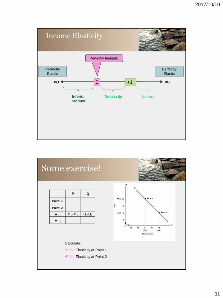
Income Elasticity

0 +1

Inferior

product

Necessity Luxury

Perfectly

Elastic

Perfectly

Elastic

∞ ∞

Perfectly Inelastic

P Q

Point: 1

Point: 2

▲1,2 P 1- P 2 Q1-Q2

▲1,2

Calculate:

•Price Elasticity at Point 1

•Price Elasticity at Point 2

Some exercise!

2017/10/10

12

Some exercise!

Question:

• Italians are choosing between two

destinations – Morocco and Tunisia. Use

the information in the table to determine

whether these two destinations are

complements or substitutes?

Answer:

Morocco Tunisia

Price (p) Quantity (x) Price (p) Quantity (x)

6 500 16 300

10 400 20 220

• 𝑒𝑚𝑜𝑟𝑜𝑐𝑐𝑜 =%∆𝑥𝑚𝑜𝑟𝑜𝑐𝑐𝑜

%∆𝑝𝑡𝑢𝑛𝑖𝑠𝑖𝑎

Some exercise!

Question:

• If Maurizio receives an

18% increase in salary

and his income demand

elasticity for yoghurt is

-2.5. How much does the

quantity of yoghurt he

demand change? What

type of product is yoghurt

to Maurizio?

Answer:

• 𝑒𝑦 =%∆𝑥

%∆𝑚

2017/10/10

13

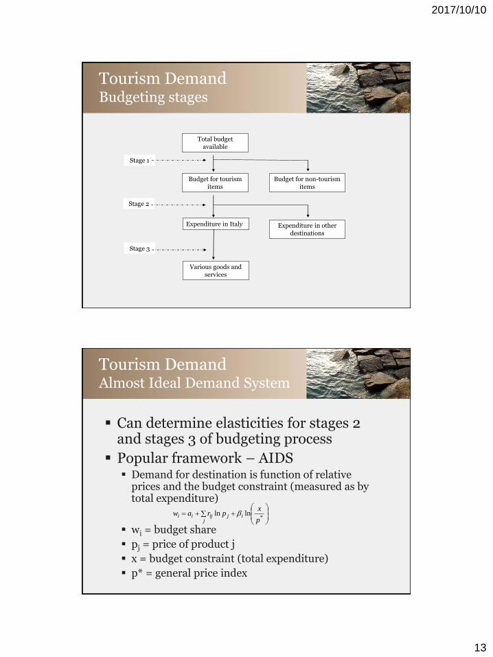
Tourism DemandBudgeting stages

Total budget available

Budget for tourism items

Budget for non-tourism items

Expenditure in Italy Expenditure in other destinations

Stage 1

Stage 2

Stage 3

Various goods and services

Can determine elasticities for stages 2 and stages 3 of budgeting process

Popular framework – AIDS Demand for destination is function of relative

prices and the budget constraint (measured as by total expenditure)

wi = budget share

pj = price of product j

x = budget constraint (total expenditure)

p* = general price index

Tourism DemandAlmost Ideal Demand System

jijijii

p

xpraw

*lnln

2017/10/10

14

Change in price

x1

e2

x2

y2

ec

Destination B

Destination A

y1

u1

u2

B1

e1

B2

xc

Expenditure elasticity

Uncompensated own-price elasticity

Uncompensated cross-price elasticity

Compensated own-price elasticity

Compensated cross-price elasticity

Elasticities

1

i

ii w

n

1

ii

iiii w

re

i

ji

i

ijij w

w

w

re

iiiiii nwee *

ijijij nwee *

2017/10/10

15

Case StudyUS demand for European destinations

• Han, Durbarry and Sinclair studies US demand for top 4 European destinations– France, Italy, Spain, UK

• First decision-making in Step 2:– Other versus top 4 European destinations

• Second decision-making in Step 2:– Allocate between the 4 destinations

–wi is ratio of expenditure in destination i relative to expenditure on all 4 destinations

– estimated system of equations using SUR method

Case StudyUS demand for European destinations

Uncompensated elasticitiesExp.elasticity

Own-price

Cross-price

France Italy UK Spain

France0.206 1.317 -1.755 - 0.748 -0.143 -0.167

Italy0.257 1.249 -2.083 0.614 - -0.090 0.310

UK0.441 0.769 -0.892 0.046 0.071 - 0.006

Spain0.0096 0.718 -1.554 -0.236 0.966 0.052 -

2017/10/10

16

Some information about Italian outbound tourism 23 million Italians travelled abroad (2004) Is one of top 10 international tourism spenders

(US$22.4 bn. in 2005) Most visited destinations:

FranceGermanySpainUK

Some facts:Spend increasingly more nights in Spain and UK, and less in

France and GermanySpend increasingly more in Germany and UK and less in

Spain and France

Case StudyOutbound Italian tourism demand

Case StudyOutbound Italian tourism demand

Uncompensated elasticitiesExp.elasticity

Own-price

Cross-price

France Germany UK Spain

France 0.988 -8.717 - 5.052 0.517 2.169

Germany 0.849 -8.593 7.168 - -0.863 1.448

UK 1.124 -0.829 0.704 -0.950 - -0.049

Spain 1.172 -5.817 3.226 1.481 -0.062 -

2017/10/10

17

Case StudyHong Kong tourist expenditure

• Focus on 3rd stage of decision-making of tourists – between products in the destination:

– Shopping

– Meals

– Hotels

• Expenditure patterns of 8 top markets of HK:

– China, South Korea, Japan, Singapore, Taiwan

– UK, USA, Australia

Case StudyHong Kong tourist expenditure - UK

Compensated elasticitiesExp.elasticity

Own- and Cross-price

Shopping Hotel Meals

Shopping 1.330* -0.588 0.392* -0.332

Hotel 0.784* 0.245* -0.416* 0.100*

Meals 0.464* -0.632 0.301* -0.593

2017/10/10

18

Case StudyHong Kong tourist expenditure - China

Compensated elasticitiesExp.elasticity

Own- and Cross-price

Shopping Hotel Meals

Shopping 0.867* -0.850* 0.155* 0.016

Hotel 1.444* 0.634* -0.721* 0.285*

Meals 0.977* 0.082 0.349* 2.150*