27
Lecture 3: Business Values Discounted Cash flow, Section 1.3 © 2004, Lutz Kruschwitz and Andreas Löffler
| Date post: | 18-Dec-2015 |
| Category: |
Documents |
| Upload: | neal-walker |
| View: | 221 times |
| Download: | 1 times |

Lecture 3: Business Values
Discounted Cash flow, Section 1.3
© 2004, Lutz Kruschwitz and Andreas Löffler

1.3.1 Trade and payment datesThe time structure of the
model:
1. Buy in t-1 pay
price.
2. Hold until t receive
dividend .
3. Sell (and buy again) in t
receive (and pay) price .
1tV
tV
Notice that the investor receives dividend shortly before t (the selling date).
tFCF
tFCF

1.3.1 A riskless worldWhat should happen if the future where certain?
In a certain world that is free of arbitrage wemust have
Otherwise, if for example
take loan, buy share in t, wait until t+1, get dividend and sell share
get infinitely rich without any cost.
1 1 .1t t
tf
FCF VV
r
1 1 (1 )t t f tFCF V r V

1.3.1 A risky world
In a risky world we have
What is absence of arbitrage now?
1
110 up,
90 down.tFCF
1 1
1t t
tf
E FCF VV
r
The account of the largest takeover in Wall Street history...

1.3.1 Three roads lead to Rome
Certainty equivalent
Risk-neutral probabilities
Risk premium
certainty equivalent
1 1 risk adjust n
1
me tt t t
tf
E FCF VV
r
F

1.3.1 Three roads lead to Rome
Certainty equivalent
Risk premium
Risk-neutral probabilities
1 1
cost of capital
risk pr1 emiumt t t
tf
E FCF VV
r
F

1.3.1 Three roads lead to Rome
Certainty equivalent
Risk premium
Risk-neutral probabilities
1 1
1t t t
tf
QE FCF VV
r
F

1.3.1 Roads to Rome: example
We are going to illustrate the three roads by using the following example:
And rf = 0.05. Because the cash flows have expectation
The value V0 will be less than
0.5 110 0.5 90 100,
10095.24.
1.05

1.3.1 Certainty Equivalent
If we assume a utility function
Then the «certainty equivalent» (CEQ)
and hence the price of the asset is given
by
( )u x x
0
0.5 110 0.5 90
99.75
99.7595.
1 1.05f
CEQ
CEQ
CEQV
r
Daniel Bernoulli, founder of
utility theory

1.3.1 Risk Premium
Valuation with a «risk premium» uses another idea: we modify
the denominator
Using the numbers of the example we get
0
0
1000.00263
1 0.05100
95.1 0.05 0.00263
V zz
V
1 1
0 .1 f
E FCF VV
r z

1.3.1 Risk-neutral ProbabilitesWith «risk-neutral probabilities» the probabilities pu=0.5 and
pd=0.5 are modified. The question is: find qu and qd such that
Holds.
Answer:
We turn to this approach in more detail!
! 1 1
0 1
Q
f
E FCF VV
r
110 9095
1 0.05
110 1 9095
1 0.050.4875, 0.5125.
u d
u u
u d
q q
q q
q q
1.3.2 Cost of capital
Cost of capital is
definitely a key concept.
But: how is it precisely
defined?

1.3.2 Cost of capital – alternative definitions
There are several alternative definitions of cost of capital in a multi-period context:
• cost of capital =Def «Yields»• cost of capital =Def «Discount rates»• cost of capital =Def «Expected returns»• cost of capital =Def «Opportunity costs»
Are all definitions identical? We will show later: not necessarily!

1.3.2 Cost of capital is an expected return
Which definition is useful for our purpose? The following
definition turns out to be appropriate
Definition 1.1 (cost of capital): The cost of capital of a
firm is the conditional expected return
1 11.
t t t
tt
E FCF Vk
V
F

1.3.2 Shortcoming of definition
This appropriate definition has a
disadvantage: kt could be uncertain.
And you cannot discount with
uncertain cost of capital!
Another (big) assumption is necessary: from now on this cost of capital should be certain.
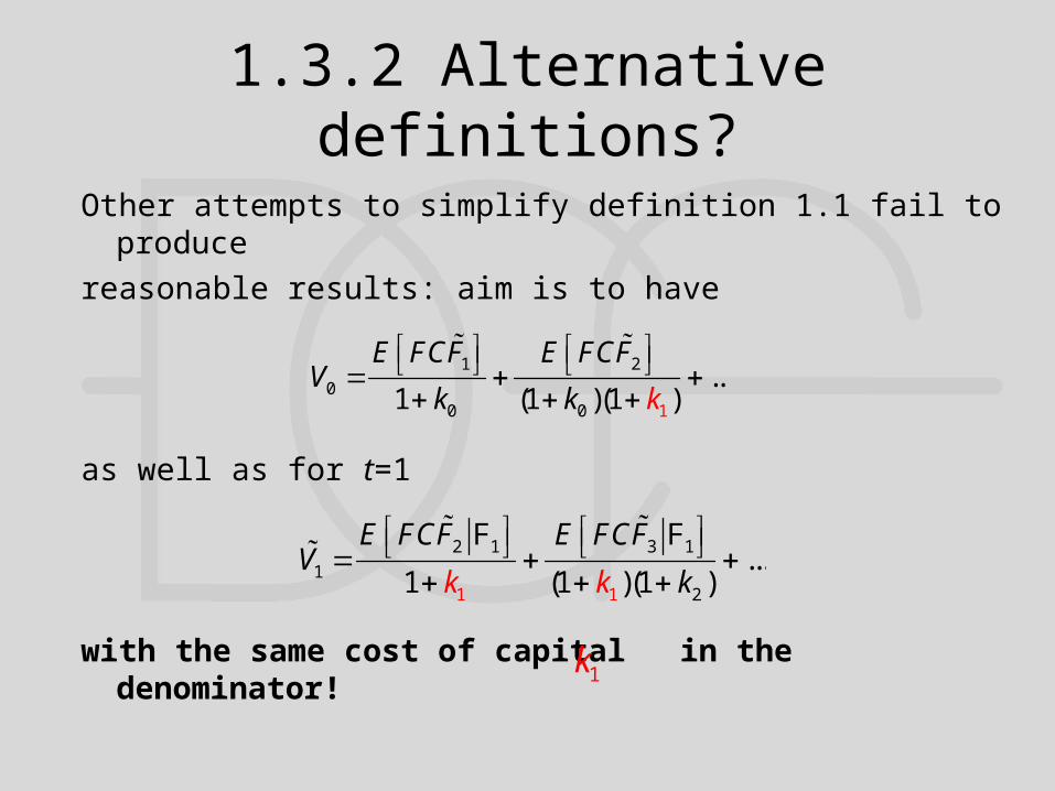
1.3.2 Alternative definitions?
Other attempts to simplify definition 1.1 fail to produce
reasonable results: aim is to have
as well as for t=1
with the same cost of capital in the denominator!
1
1 2
00 0
...1 (1 )(1 )
E FCF E FCFV
k k k
2 1 3 1
21 11 ...
1 (1 )(1 )
E FCF E FCFV
kk k
F F
1k

1.3.3 Market value
Theorem 1.1 (market value): When cost of capital is
deterministic, then
Notice that the lefthand side and the righthand side as well
can be uncertain for t>0.
1 1
.(1 )...(1 )
Ts t
ts t t s
E FCFV
k k
F

1.3.3 Proof of Theorem 1.1
Start with a reformulation of Definition 1.1,
Now use the similar relation for and plug in,
1 1.
1t t t
tt
E FCF VV
k
F
2 2 1
11 1
.1
t t t
t t
tt
t
E FCF
V
E FCF V
k
k
F
F
1tV

1.3.3 Proof (continued)
Costs of capital are deterministic, use rule 2 (linearity)
Rule 4 (iterated expectation) gives
2 1 2 11
1 1
.1 1 1 1 1
t t t t t tt t
tt t t t t
E E FCF E E VE FCFV
k k k k k
F F F FF
1 2 1 2 1
1 1
.1 1 1 1 1
t t t t t t
tt t t t t
E FCF E FCF E VV
k k k k k
F F F
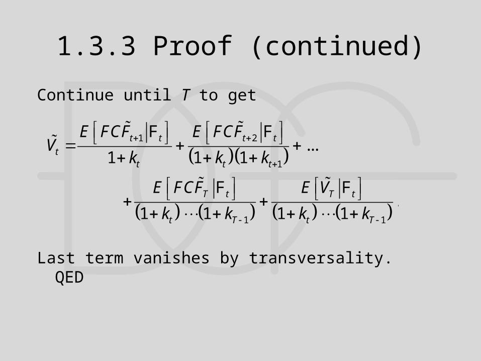
1.3.3 Proof (continued)
Continue until T to get
Last term vanishes by transversality. QED
1 2
1
1 1
...1 1 1
.1 1 1 1
t t t t
tt t t
T t T t
t T t T
E FCF E FCFV
k k k
E FCF E V
k k k k
F F
F F

1.3.4 Fundamental Theorem
Let us turn back to risk-neutral probability Q: does Q always
exist?
This is not a trivial question: the numbers qu and qd must be
between 0 and 1! For example, would not be
considered as «probabilities».
Theorem 1.2 (Fundamental Theorem): If the markets are free of arbitrage, there is a probability Q such that for all claims
1 1.
1Q t t t
tf
E FCF VV
r
F
, 2,1u dq q

1.3.4 Fundamental theorem
What about a proof? Forget it.1
How to get Q for valuation of firms? No idea.
So why is this helpful? We will see (much) later.
Is there at least an interpretation of Q? Yes!
1If you cannot resist: see further literature

1.3.4 Risk-neutrality of Q
Why do we call Q a risk-neutral probability?
Look at the following:
1 1
1 1
1 1
1 1
1 fundamental theorem
1 rule 5
1 rule 3
1 rule 2.
Q t t t
ft
t tf Q t
t
t tf Q t Q t
t
t tf Q t
t
E FCF Vr
V
FCF Vr E
V
FCF Vr E E
V
FCF Vr E
V
F
F
F F
F
return on holding a share

1.3.4 Intuition of Q
The last equation
simply says: if we change our probabilites to Q, any security
has expected return rf.
Or: the world is risk-neutral under Q .
returnf Q tr E F

1.3.4 Uniqueness of Q
Is Q unique? Or can the value of the company depend on Q?
If the cash flows of the firm can be duplicated by traded assets
(market is complete) then any Q will lead to the same value.
Proof: Forget this as well...

1.3.4 Two assumptions
From now on two assumptions will always hold:
Assumption 1.1: The markets are free of arbitrage.
Assumption 1.2: The cash flows of the firm can be duplicated
by traded assets.
The risk-neutral probability Q exists and is (in some sense)
unique.

Summary
Costs of capital are conditional expected returns.
Costs of capital must be deterministic.
If markets are arbitrage free a «risk-neutral probability
measure» Q exists.
When using this probability Q the world is risk-neutral.


