Lecture 3: Constrained Optimizationktcarlb/opt_class/OPT_Lecture3.pdf · Lecture 3: Constrained...

Outline and terminologiesFirst-order optimality: Unconstrained problems

First-order optimality: Constrained problemsSecond-order optimality conditions

Algorithms

Lecture 3: Constrained Optimization

Kevin Carlberg

Stanford University

July 31, 2009

Kevin Carlberg Lecture 3: Constrained Optimization



Algorithms

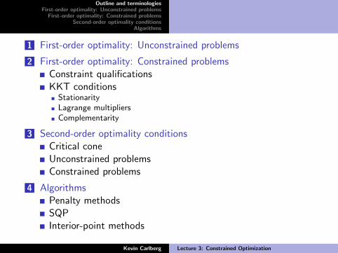
1 First-order optimality: Unconstrained problems

2 First-order optimality: Constrained problemsConstraint qualificationsKKT conditions

StationarityLagrange multipliersComplementarity

3 Second-order optimality conditionsCritical coneUnconstrained problemsConstrained problems

4 AlgorithmsPenalty methodsSQPInterior-point methods




Algorithms

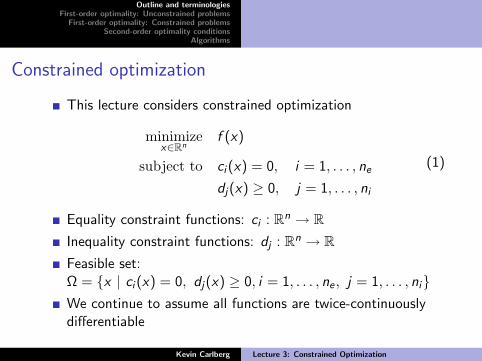
Constrained optimization

This lecture considers constrained optimization

minimizex∈Rn

f (x)

subject to ci (x) = 0, i = 1, . . . , ne

dj(x) ≥ 0, j = 1, . . . , ni

(1)

Equality constraint functions: ci : Rn → RInequality constraint functions: dj : Rn → RFeasible set:Ω = x | ci (x) = 0, dj(x) ≥ 0, i = 1, . . . , ne , j = 1, . . . , niWe continue to assume all functions are twice-continuouslydifferentiable




Algorithms

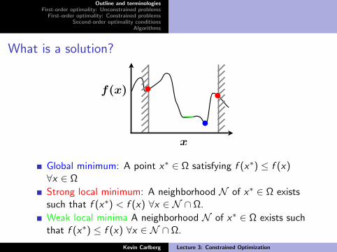
What is a solution?

x

f(x)

Global minimum: A point x∗ ∈ Ω satisfying f (x∗) ≤ f (x)∀x ∈ Ω

Strong local minimum: A neighborhood N of x∗ ∈ Ω existssuch that f (x∗) < f (x) ∀x ∈ N ∩ Ω.

Weak local minima A neighborhood N of x∗ ∈ Ω exists suchthat f (x∗) ≤ f (x) ∀x ∈ N ∩ Ω.




Algorithms

Convexity

As with the unconstrained case, conditions hold where any localminimum is the global minimum:

f (x) convex

ci (x) affine (ci (x) = Aix + bi ) for i = 1, . . . , ne

dj(x) convex for j = 1, . . . , ni




Algorithms

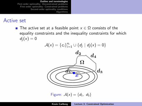
Active set

The active set at a feasible point x ∈ Ω consists of theequality constraints and the inequality constraints for whichdj(x) = 0

A(x) = cinii=1 ∪ dj | dj(x) = 0

x

f(x)

d2

d3d1

!d4

x

Figure: A(x) = d1, d3




Algorithms

Formulation of first-order conditions

Wordsto first-order, the function cannot decrease by moving in feasible

directions↓

Geometric descriptiondescription using the geometry of the feasible set

↓Algebraic description

description using the equations of the active constraints

The algebraic description is required to actually solveproblems (use equations!)




Algorithms

First-order conditions for unconstrained problems

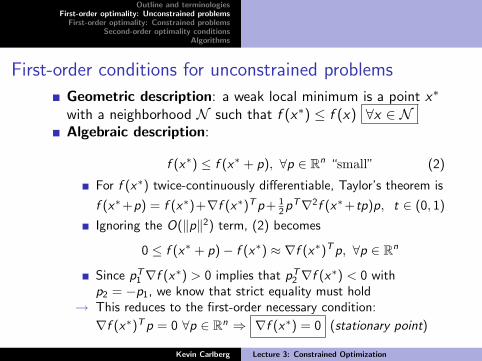
Geometric description: a weak local minimum is a point x∗

with a neighborhood N such that f (x∗) ≤ f (x) ∀x ∈ NAlgebraic description:

f (x∗) ≤ f (x∗ + p), ∀p ∈ Rn “small” (2)

For f (x∗) twice-continuously differentiable, Taylor’s theorem is

f (x∗+p) = f (x∗)+∇f (x∗)T p + 12 pT∇2f (x∗+tp)p, t ∈ (0, 1)

Ignoring the O(‖p‖2) term, (2) becomes

0 ≤ f (x∗ + p)− f (x∗) ≈ ∇f (x∗)T p, ∀p ∈ Rn

Since pT1 ∇f (x∗) > 0 implies that pT

2 ∇f (x∗) < 0 withp2 = −p1, we know that strict equality must hold

→ This reduces to the first-order necessary condition:

∇f (x∗)T p = 0 ∀p ∈ Rn ⇒ ∇f (x∗) = 0 (stationary point)




Algorithms

Constraint qualificationsKKT conditions

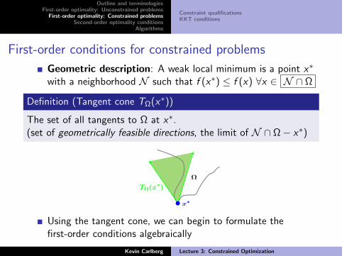
First-order conditions for constrained problems

Geometric description: A weak local minimum is a point x∗

with a neighborhood N such that f (x∗) ≤ f (x) ∀x ∈ N ∩ Ω

Definition (Tangent cone TΩ(x∗))

The set of all tangents to Ω at x∗.(set of geometrically feasible directions, the limit of N ∩ Ω− x∗)

T!(x!)

x!

!

Using the tangent cone, we can begin to formulate thefirst-order conditions algebraically




Algorithms


First-order conditions for constrained problems

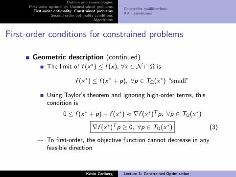
Geometric description (continued)

The limit of f (x∗) ≤ f (x), ∀x ∈ N ∩ Ω is

f (x∗) ≤ f (x∗ + p), ∀p ∈ TΩ(x∗) “small”

Using Taylor’s theorem and ignoring high-order terms, thiscondition is

0 ≤ f (x∗ + p)− f (x∗) ≈ ∇f (x∗)T p, ∀p ∈ TΩ(x∗)

∇f (x∗)T p ≥ 0, ∀p ∈ TΩ(x∗) (3)

→ To first-order, the objective function cannot decrease in anyfeasible direction




Algorithms


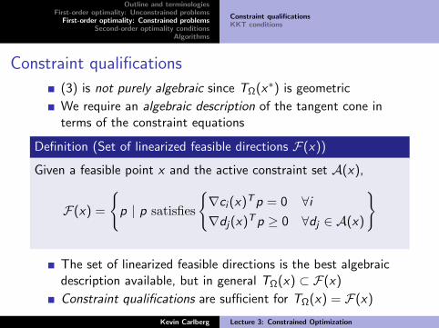
Constraint qualifications

(3) is not purely algebraic since TΩ(x∗) is geometric

We require an algebraic description of the tangent cone interms of the constraint equations

Definition (Set of linearized feasible directions F(x))

Given a feasible point x and the active constraint set A(x),

F(x) =

p | p satisfies

∇ci (x)T p = 0 ∀i

∇dj(x)T p ≥ 0 ∀dj ∈ A(x)

The set of linearized feasible directions is the best algebraicdescription available, but in general TΩ(x) ⊂ F(x)

Constraint qualifications are sufficient for TΩ(x) = F(x)




Algorithms


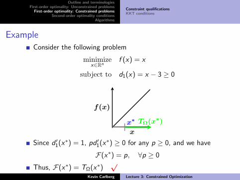
ExampleConsider the following problem

minimizex∈Rn

f (x) = x

subject to d1(x) = x − 3 ≥ 0

x

f(x)

x! T!(x!)

x

y

!x+3

!2 !1 0 1 2 3 4 5 6

!3

!2

!1

0

1

2

3

4

5

6

x!

x1

x2

!d1(x!) !f(x!)

x

y

!x+3

!2 !1 0 1 2 3 4 5 6

!3

!2

!1

0

1

2

3

4

5

6

x!

x1

x2

x

!f(x)

!d1(x)

feasible descent

directions

Since d ′1(x∗) = 1, pd ′1(x∗) ≥ 0 for any p ≥ 0, and we have

F(x∗) = p, ∀p ≥ 0

Thus, F(x∗) = TΩ(x∗)√




Algorithms


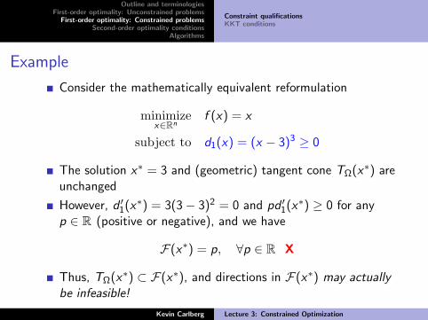
Example

Consider the mathematically equivalent reformulation

minimizex∈Rn

f (x) = x

subject to d1(x) = (x − 3)3 ≥ 0

The solution x∗ = 3 and (geometric) tangent cone TΩ(x∗) areunchanged

However, d ′1(x∗) = 3(3− 3)2 = 0 and pd ′1(x∗) ≥ 0 for anyp ∈ R (positive or negative), and we have

F(x∗) = p, ∀p ∈ R X

Thus, TΩ(x∗) ⊂ F(x∗), and directions in F(x∗) may actuallybe infeasible!




Algorithms


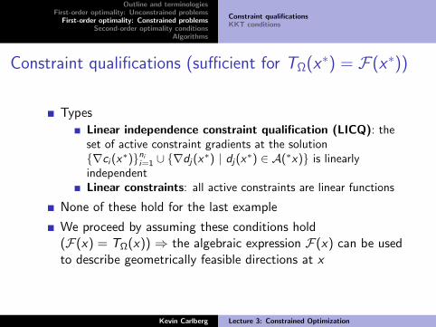
Constraint qualifications (sufficient for TΩ(x∗) = F(x∗))

Types

Linear independence constraint qualification (LICQ): theset of active constraint gradients at the solution∇ci (x∗)ni

i=1 ∪ ∇dj(x∗) | dj(x∗) ∈ A(∗x) is linearlyindependentLinear constraints: all active constraints are linear functions

None of these hold for the last example

We proceed by assuming these conditions hold(F(x) = TΩ(x)) ⇒ the algebraic expression F(x) can be usedto describe geometrically feasible directions at x




Algorithms


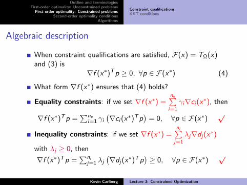
Algebraic description

When constraint qualifications are satisfied, F(x) = TΩ(x)and (3) is

∇f (x∗)T p ≥ 0, ∀p ∈ F(x∗) (4)

What form ∇f (x∗) ensures that (4) holds?

Equality constraints: if we set ∇f (x∗) =ne∑i=1

γi∇ci (x∗), then

∇f (x∗)T p =∑ne

i=1 γi

(∇ci (x∗)T p

)= 0, ∀p ∈ F(x∗)

√

Inequality constraints: if we set ∇f (x∗) =ni∑

j=1λj∇dj(x∗)

with λj ≥ 0, then

∇f (x∗)T p =∑ni

j=1 λj

(∇dj(x∗)T p

)≥ 0, ∀p ∈ F(x∗)

√




Algorithms


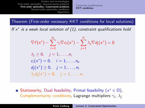
Theorem (First-order necessary KKT conditions for local solutions)

If x∗ is a weak local solution of (1), constraint qualifications hold

∇f (x∗)−ne∑i=1

γi∇ci (x∗)−ni∑

j=1

λj∇dj(x∗) = 0

λj ≥ 0, j = 1, . . . , ni

ci (x∗) = 0, i = 1, . . . , ne

dj(x∗) ≥ 0, j = 1, . . . , ni

λjdj(x∗) = 0, j = 1, . . . , ni

Stationarity, Dual feasibility, Primal feasibility (x∗ ∈ Ω),Complementarity conditions, Lagrange multipliers γi , λj




Algorithms


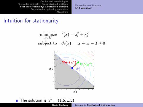
Intuition for stationarity

minimizex∈Rn

f (x) = x21 + x2

2

subject to d1(x) = x1 + x2 − 3 ≥ 0x

f(x)

x! T!(x!)

x

y

!x+3

!2 !1 0 1 2 3 4 5 6

!3

!2

!1

0

1

2

3

4

5

6

x!

x1

x2

!d1(x!) !f(x!)

The solution is x∗ = (1.5, 1.5)Kevin Carlberg Lecture 3: Constrained Optimization



Algorithms


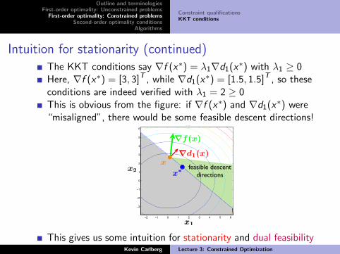
Intuition for stationarity (continued)The KKT conditions say ∇f (x∗) = λ1∇d1(x∗) with λ1 ≥ 0Here, ∇f (x∗) = [3, 3]T , while ∇d1(x∗) = [1.5, 1.5]T , so theseconditions are indeed verified with λ1 = 2 ≥ 0This is obvious from the figure: if ∇f (x∗) and ∇d1(x∗) were“misaligned”, there would be some feasible descent directions!

x

f(x)

x! T!(x!)

x

y

!x+3

!2 !1 0 1 2 3 4 5 6

!3

!2

!1

0

1

2

3

4

5

6

x!

x1

x2

!d1(x!) !f(x!)

x

y

!x+3

!2 !1 0 1 2 3 4 5 6

!3

!2

!1

0

1

2

3

4

5

6

x!

x1

x2

x

!f(x)

!d1(x)

feasible descent

directions

This gives us some intuition for stationarity and dual feasibilityKevin Carlberg Lecture 3: Constrained Optimization



Algorithms


Lagrangian

Definition (Lagrangian)

The Lagrangian for (1) is

L(x , γ, λ) = f (x)−ne∑i=1

γici (x)−ni∑

j=1λjdj(x)

Stationarity in the sense of KKT is equivalent to stationarityof the Lagrangian with respect to x :

Lx(x , γ, λ) = ∇f (x)−ne∑i=1

γi∇ci (x)−ni∑

j=1

λj∇dj(x)

KKT stationarity ⇔ Lx(x∗, γ, λ) = 0




Algorithms


Lagrange multipliers

Lagrange multipliers γi and λj arise in constrainedminimization problems

They tell us something about the sensitivity of f (x∗) to thepresence of their constraints. γi and λj indicate how hard f is“pushing” or “pulling” the solution against ci and dj .

If we perturb the right-hand side of the i th equality constraintso that ci (x) ≥ −ε‖∇ci (x∗)‖, then

df (x∗(ε))

dε= −γi‖∇ci (x∗)‖.

If the j th inequality is perturbed so dj(x) ≥ −ε‖∇dj(x∗)‖,

df (x∗(ε))

dε= −λj‖∇di (x∗)‖.




Algorithms


Constraint classification

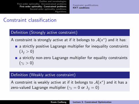
Definition (Strongly active constraint)

A constraint is strongly active at if it belongs to A(x∗) and it has:

a strictly positive Lagrange multiplier for inequality constraints(λj > 0)

a strictly non-zero Lagrange multiplier for equality constraints(γi > 0)

Definition (Weakly active constraint)

A constraint is weakly active at if it belongs to A(x∗) and it has azero-valued Lagrange multiplier (γi = 0 or λj = 0)




Algorithms


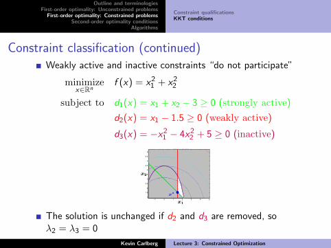
Constraint classification (continued)Weakly active and inactive constraints “do not participate”

minimizex∈Rn

f (x) = x21 + x2

2

subject to d1(x) = x1 + x2 − 3 ≥ 0 (strongly active)

d2(x) = x1 − 1.5 ≥ 0 (weakly active)

d3(x) = −x21 − 4x2

2 + 5 ≥ 0 (inactive)

x1

x2

!1 0 1 2 3 4 5

1

1.5

2

2.5

3

3.5

4

4.5

5

5.5

6

x

y

x = !1 sqrt(!1/4 x2+20/4), y = k

x!

The solution is unchanged if d2 and d3 are removed, soλ2 = λ3 = 0




Algorithms


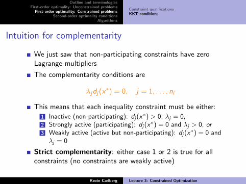
Intuition for complementarity

We just saw that non-participating constraints have zeroLagrange multipliers

The complementarity conditions are

λjdj(x∗) = 0, j = 1, . . . , ni

This means that each inequality constraint must be either:

1 Inactive (non-participating): dj(x∗) > 0, λj = 0,2 Strongly active (participating): dj(x∗) = 0 and λj > 0, or3 Weakly active (active but non-participating): dj(x∗) = 0 andλj = 0

Strict complementarity: either case 1 or 2 is true for allconstraints (no constraints are weakly active)




Algorithms

Critical coneUnconstrained problemsConstrained problems

Second-order optimality conditions

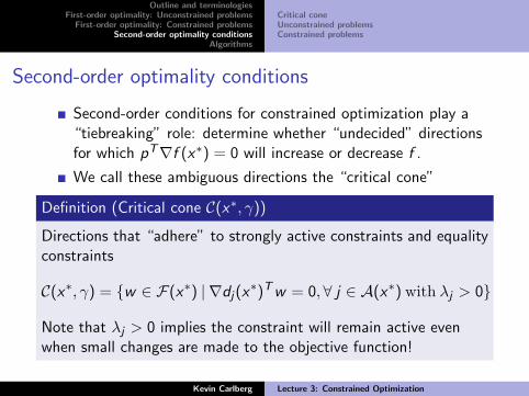
Second-order conditions for constrained optimization play a“tiebreaking” role: determine whether “undecided” directionsfor which pT∇f (x∗) = 0 will increase or decrease f .

We call these ambiguous directions the “critical cone”

Definition (Critical cone C(x∗, γ))

Directions that “adhere” to strongly active constraints and equalityconstraints

C(x∗, γ) = w ∈ F(x∗) | ∇dj(x∗)T w = 0,∀ j ∈ A(x∗) with λj > 0

Note that λj > 0 implies the constraint will remain active evenwhen small changes are made to the objective function!




Algorithms


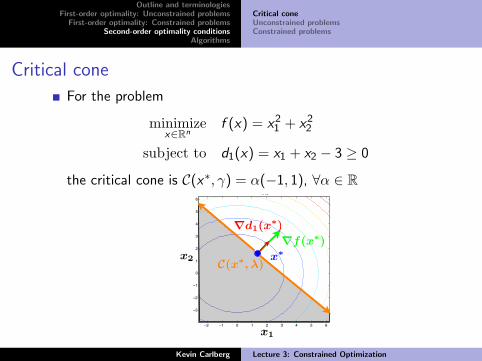
Critical cone

For the problem

minimizex∈Rn

f (x) = x21 + x2

2

subject to d1(x) = x1 + x2 − 3 ≥ 0

the critical cone is C(x∗, γ) = α(−1, 1), ∀α ∈ R

x

y

!x+3

!2 !1 0 1 2 3 4 5 6

!3

!2

!1

0

1

2

3

4

5

6

x!

x1

x2

!d1(x!)!f(x!)

C(x!, !)




Algorithms


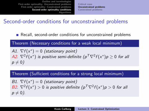
Second-order conditions for unconstrained problems

Recall, second-order conditions for unconstrained problems

Theorem (Necessary conditions for a weak local minimum)

A1. ∇f (x∗) = 0 (stationary point)A2. ∇2f (x∗) is positive semi-definite (pT∇2f (x∗)p ≥ 0 for allp 6= 0)

Theorem (Sufficient conditions for a strong local minimum)

B1. ∇f (x∗) = 0 (stationary point)B2. ∇2f (x∗) > 0 is positive definite (pT∇2f (x∗)p > 0 for allp 6= 0).




Algorithms


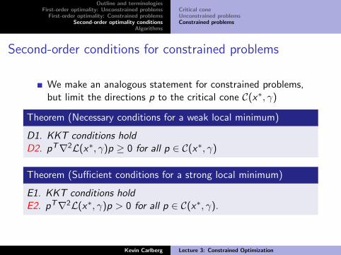
Second-order conditions for constrained problems

We make an analogous statement for constrained problems,but limit the directions p to the critical cone C(x∗, γ)

Theorem (Necessary conditions for a weak local minimum)

D1. KKT conditions holdD2. pT∇2L(x∗, γ)p ≥ 0 for all p ∈ C(x∗, γ)

Theorem (Sufficient conditions for a strong local minimum)

E1. KKT conditions holdE2. pT∇2L(x∗, γ)p > 0 for all p ∈ C(x∗, γ).




Algorithms


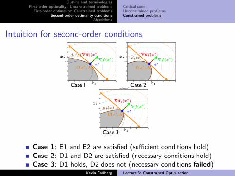
Intuition for second-order conditions

x!

x1

x2!d1(x!)

!f(x!)

x

y

(x+y)2+3 (x!y)

2

0 1 2 3 4 5 6 7 80

1

2

3

4

5

6

7

8

x!

x1

x2!d1(x!)

!f(x!)

x

y

(x+y)2+3 (x!y)

2

0 1 2 3 4 5 6 7 80

1

2

3

4

5

6

7

8

x!

x1

x2!d1(x!)

!f(x!)

x

y

(x+y)2+3 (x!y)

2

0 1 2 3 4 5 6 7 80

1

2

3

4

5

6

7

8

C(x!, !) C(x!, !)

C(x!, !)

d1(x)d1(x)

d1(x)

Case I Case 2

Case 3

Case 1: E1 and E2 are satisfied (sufficient conditions hold)Case 2: D1 and D2 are satisfied (necessary conditions hold)Case 3: D1 holds, D2 does not (necessary conditions failed)




Algorithms


Next

We now know how to correctly formulate constrainedoptimization problems and how to verify whether a givenpoint x could be a solution (necessary conditions) or iscertainly a solution (sufficient conditions)

Next, we learn algorithms that are use to compute solutionsto these problems




Algorithms

Penalty methodsSQPInterior-point methods

Constrained optimization algorithms

Linear programming (LP)

Simplex method: created by Dantzig in 1947. Birth of themodern era in optimizationInterior-point methods

Nonlinear programming (NLP)

Penalty methodsSequential quadratic programming methodsInterior-point methods

Almost all these methods rely strongly on line-search andtrust region methodologies for unconstrained optimization




Algorithms


Penalty methods

Penalty methods combine the objective function andconstraints

minimizex∈Rn

f (x) s.t. ci (x) = 0, i = 1, . . . , ni

↓

minimizex∈Rn

f (x) +µ

2

ni∑i=1

c2i (x)

A sequence of unconstrained problems is then solved for µincreasing




Algorithms


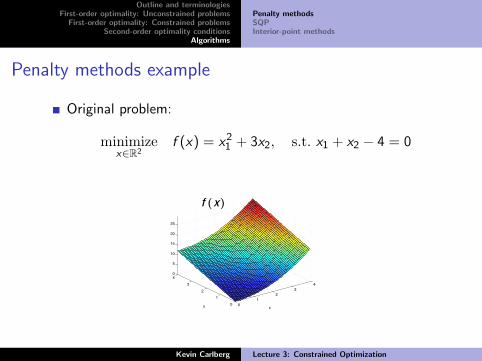
Penalty methods example

Original problem:

minimizex∈R2

f (x) = x21 + 3x2, s.t. x1 + x2 − 4 = 0

0

1

2

3

4

0

1

2

3

40

5

10

15

20

25

x

x2+3 y

y

f (x)




Algorithms


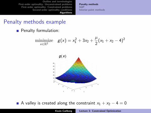
Penalty methods example

Penalty formulation:

minimizex∈R2

g(x) = x21 + 3x2 +

µ

2(x1 + x2 − 4)2

0

1

2

3

4

0

1

2

3

40

5

10

15

20

25

x

x2+3 y

y

f ( x )

0

1

2

3

4

0

1

2

3

40

10

20

30

40

50

60

x

x2+3 y+µ (x+y! 4)

2

y

g(x)

A valley is created along the constraint x1 + x2 − 4 = 0




Algorithms


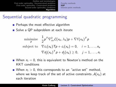
Sequential quadratic programming

Perhaps the most effective algorithm

Solve a QP subproblem at each iterate

minimizep

1

2pT∇2

xxL(xk , λk)p +∇f (xk)T p

subject to ∇ci (xk)Tp + ci (xk) = 0, i = 1, . . . , ne

∇dj(xk)T p + dj(xk) ≥ 0, j = 1, . . . , ni

When ni = 0, this is equivalent to Newton’s method on theKKT conditions

When ni > 0, this corresponds to an “active set” method,where we keep track of the set of active constraints A(xk) ateach iteration




Algorithms


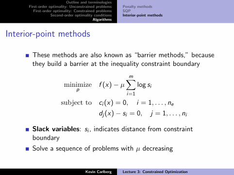
Interior-point methods

These methods are also known as “barrier methods,” becausethey build a barrier at the inequality constraint boundary

minimizep

f (x)− µm∑

i=1

log si

subject to ci (x) = 0, i = 1, . . . , ne

dj(x)− si = 0, j = 1, . . . , ni

Slack variables: si , indicates distance from constraintboundary

Solve a sequence of problems with µ decreasing




Algorithms


Interior-point methods example

Original problem:

minimizex∈R2

f (x) = x21 + 3x2, s.t. − x1 − x2 + 4 ≥ 0

0

1

2

3

4

0

1

2

3

40

5

10

15

20

25

x

x2+3 y

y

f (x)




Algorithms


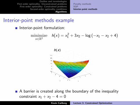
Interior-point methods example

Interior-point formulation:

minimizex∈R2

h(x) = x21 + 3x2 − log (−x1 − x2 + 4)

A barrier is created along the boundary of the inequalityconstraint x1 + x2 − 4 = 0




Algorithms


Summary

We now now something about:

Modeling and classifying unconstrained and constrainedoptimization problemsIdentifying local minima (necessary and sufficient conditions)Solving the problem using numerical optimization algorithms

We next consider the case of PDE-constrained optimization,which enables us to use to tools learned earlier (finiteelements) in optimal design and control settings, for example


Date post:	26-May-2018
Category:	Documents
Upload:	dodang
View:	219 times
Download:	1 times

Lecture 3: Constrained Optimizationktcarlb/opt_class/OPT_Lecture3.pdf · Lecture 3: Constrained...

Documents