– 3 – 2016-04-25 – main – Softwaretechnik / Software-Engineering Lecture 3: Metrics Cont’d & Cost Estimation 2016-04-25 Prof. Dr. Andreas Podelski, Dr. Bernd Westphal Albert-Ludwigs-Universität Freiburg, Germany
Transcript
–3
–2
016
-04
-25
–m
ain
–
Softwaretechnik / Software-Engineering
Lecture 3: Metrics Cont’d & Cost Estimation
2016-04-25
Prof. Dr. Andreas Podelski, Dr. Bernd Westphal
Albert-Ludwigs-Universität Freiburg, Germany
Content–
3–
20
16-0
4-2
5–
Sco
nte
nt
–
2/40
• Software Metrics
• Motivation
• Vocabulary
• Requirements on Useful Metrics
• Excursion: Scales
• Example: LOC
• Other Properties of Metrics
• Subjective and Pseudo Metrics
• Discussion
• Cost Estimation
• “(Software) Economics in a Nutshell”
• Cost Estimation
• Expert’s Estimation
• The Delphi Method
• Algorithmic Estimation
• COCOMO
• Function Points
westphal
Bleistift
westphal
Bleistift
westphal
Bleistift
westphal
Bleistift
westphal
Bleistift
Recall: Pseudo-Metrics–
3–
20
16-0
4-2
5–
Sp
seu
do
con
t–
3/40
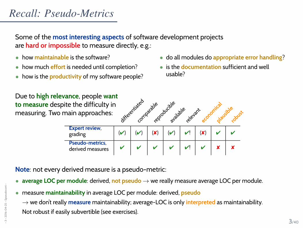
Some of the most interesting aspects of software development projectsare hard or impossible to measure directly, e.g.:
• how maintainable is the software?
• how much effort is needed until completion?
• how is the productivity of my software people?
• do all modules do appropriate error handling?
• is the documentation sufficient and wellusable?
Due to high relevance, people wantto measure despite the difficulty inmeasuring. Two main approaches:
differ
entia
ted
com
parab
lere
produc
ible
avail
able
rele
vant
econom
ical
plausib
lero
bust
Expert review,grading (✔) (✔) (✘) (✔) ✔! (✘) ✔ ✔
Pseudo-metrics,derived measures ✔ ✔ ✔ ✔ ✔! ✔ ✘ ✘
Note: not every derived measure is a pseudo-metric:
• average LOC per module: derived, not pseudo → we really measure average LOC per module.
• measure maintainability in average LOC per module: derived, pseudo
→ we don’t really measure maintainability; average-LOC is only interpreted as maintainability.
Not robust if easily subvertible (see exercises).
Can Pseudo-Metrics be Useful?–
3–
20
16-0
4-2
5–
Sp
seu
do
con
t–
4/40
• Pseudo-metrics can be useful if there is a (good) correlation (with few false positives and fewfalse negatives) between valuation yields and the property to be measured:
valuation yieldlow high
qu
alit
yhigh
false positive
×
true positive
× ×
× × ×
× ×
low
true negative
× ×
×
× ×
false negative
×
× ×
• This may strongly depend on context information:
• If LOC was (or could be made non-subvertible (→ tutorials)),then productivity could be a useful measure for, e.g., team performance.
westphal
Bleistift
westphal
Bleistift
westphal
Bleistift
westphal
Bleistift
westphal
Bleistift
westphal
Bleistift
westphal
Bleistift
Code Metrics for OO Programs (Chidamber and Kemerer, 1994)–
3–
20
16-0
4-2
5–
Sp
seu
do
con
t–
5/40
metric computation
weighted methodsper class (WMC)
n∑
i=1
ci , n = number of methods, ci = complexity of method i
depth of inheritancetree (DIT)
graph distance in inheritance tree (multiple inheritance ?)
number of childrenof a class (NOC)
number of direct subclasses of the class
coupling betweenobject classes (CBO)
CBO(C) = |Ko ∪Ki|,Ko = set of classes used by C , Ki = set of classes using C
response for a class(RFC)
RFC = |M ∪⋃
i Ri|, M set of methods of C ,Ri set of all methods calling method i
lack of cohesion inmethods (LCOM)
max(|P | − |Q|, 0), P = methods using no common attribute,Q = methods using at least one common attribute
• direct metrics: DIT, NOC, CBO; pseudo-metrics: WMC, RFC, LCOM
. . . there seems to be agreement that it is far more important to focus on empirical validation (orrefutation) of the proposed metrics than to propose new ones, . . . (Kan, 2003)
Subjective Metrics
–3
–2
016
-04
-25
–m
ain
–
6/40
Subjective Metrics–
3–
20
16-0
4-2
5–
Ssu
bje
ctiv
e–
7/40
example problems countermeasures
Statement “Thespecification isavailable.”
Terms may beambiguous,conclusions arehardly possible.
Allow only certainstatements, characterisethem precisely.
Assessment “The module iscoded in a cleverway.”
Not necessarilycomparable.
Only offer particularoutcomes; put them on an(at least ordinal) scale.
Grading “Readability isgraded 4.0.”
Subjective;grading notreproducible.
Define criteria for grades;give examples how to grade;practice on existing artefacts
(Ludewig and Lichter, 2013)
Example: A (Subjective) Metric for Maintainability–
3–
20
16-0
4-2
5–
Ssu
bje
ctiv
e–
8/40
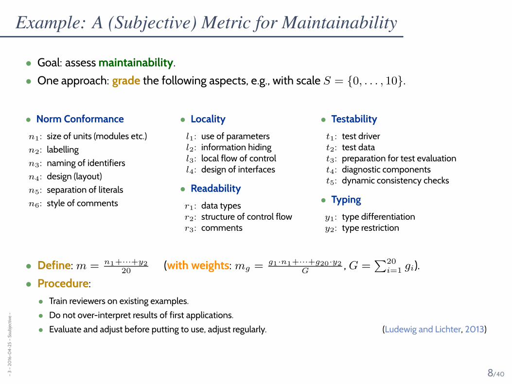
• Goal: assess maintainability.
• One approach: grade the following aspects, e.g., with scale S = {0, . . . , 10}.
• Norm Conformance
n1 : size of units (modules etc.)
n2 : labelling
n3 : naming of identifiers
n4 : design (layout)
n5 : separation of literals
n6 : style of comments
• Locality
l1 : use of parametersl2 : information hidingl3 : local flow of controll4 : design of interfaces
• Readability
r1 : data typesr2 : structure of control flowr3 : comments
• Testability
t1 : test drivert2 : test datat3 : preparation for test evaluationt4 : diagnostic componentst5 : dynamic consistency checks
• Typing
y1 : type differentiationy2 : type restriction
• Define: m = n1+···+y220
(with weights: mg = g1·n1+···+g20·y2G
, G =∑
20
i=1gi).
• Procedure:
• Train reviewers on existing examples.
• Do not over-interpret results of first applications.
• Evaluate and adjust before putting to use, adjust regularly. (Ludewig and Lichter, 2013)
westphal
Bleistift
Example: A (Subjective) Metric for Maintainability–
3–
20
16-0
4-2
5–
Ssu
bje
ctiv
e–
8/40
• Goal: assess maintainability.
• One approach: grade the following aspects, e.g., with scale S = {0, . . . , 10}.
• Norm Conformance
n1 : size of units (modules etc.)
n2 : labelling
n3 : naming of identifiers
n4 : design (layout)
n5 : separation of literals
n6 : style of comments
• Locality
l1 : use of parametersl2 : information hidingl3 : local flow of controll4 : design of interfaces
• Readability
r1 : data typesr2 : structure of control flowr3 : comments
• Testability
t1 : test drivert2 : test datat3 : preparation for test evaluationt4 : diagnostic componentst5 : dynamic consistency checks
• Typing
y1 : type differentiationy2 : type restriction
• Define: m = n1+···+y220
(with weights: mg = g1·n1+···+g20·y2G
, G =∑
20
i=1gi).
• Procedure:
• Train reviewers on existing examples.
• Do not over-interpret results of first applications.
• Evaluate and adjust before putting to use, adjust regularly. (Ludewig and Lichter, 2013)
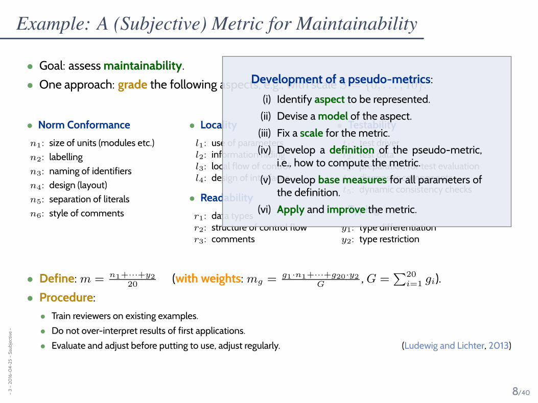
Development of a pseudo-metrics:
(i) Identify aspect to be represented.
(ii) Devise a model of the aspect.
(iii) Fix a scale for the metric.
(iv) Develop a definition of the pseudo-metric,i.e., how to compute the metric.
(v) Develop base measures for all parameters ofthe definition.
(vi) Apply and improve the metric.
The Goal-Question-Metric Approach
–3
–2
016
-04
-25
–m
ain
–
9/40
Information Overload!?–
3–
20
16-0
4-2
5–
Sgq
m–
10/40
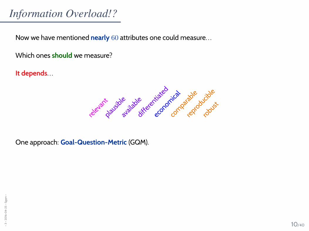
Now we have mentioned nearly 60 attributes one could measure. . .
Which ones should we measure?
It depends. . .
rele
vant
plaus
ible
avail
able
differ
entia
ted
econom
ical
com
parab
lere
produc
ible
robus
t
One approach: Goal-Question-Metric (GQM).
westphal
Bleistift
westphal
Bleistift
Goal-Question-Metric (Basili and Weiss, 1984)–
3–
20
16-0
4-2
5–
Sgq
m–
11/40
The three steps of GQM:
(i) Define the goals relevant for a project or an organisation.
(ii) From each goal, derive questionswhich need to be answered to check whether the goal is reached.
(iii) For each question, choose (or develop) metricswhich contribute to finding answers.
Being good wrt. to a certain metric is (in general) not an asset on its own.We usually want to optimise wrt. goals, not wrt. metrics.In particular critical: pseudo-metrics for quality.
Software and process measurements may yield personaldata (“personenbezogene Daten”).Their collection may be regulated by laws.
And Which Metrics Should One Use?–
3–
20
16-0
4-2
5–
Sgq
m–
12/40
And Which Metrics Should One Use?–
3–
20
16-0
4-2
5–
Sgq
m–
12/40
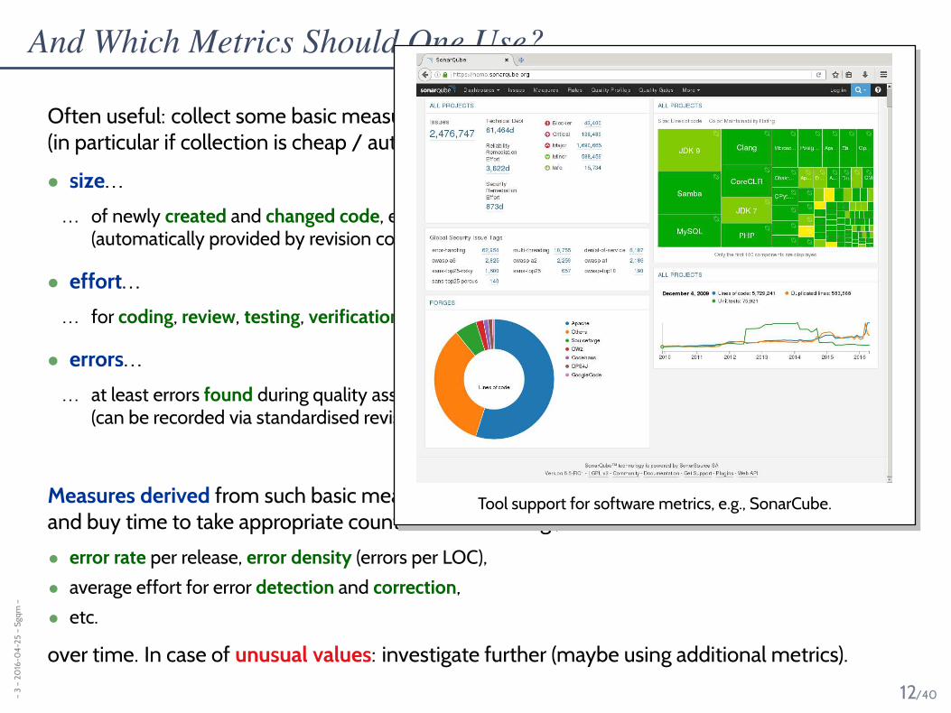
Often useful: collect some basic measures in advance(in particular if collection is cheap / automatic), e.g.:
• size. . .
. . . of newly created and changed code, etc.(automatically provided by revision control software),
• effort. . .
. . . for coding, review, testing, verification, fixing, maintenance, etc.
• errors. . .
. . . at least errors found during quality assurance, and errors reported by customer(can be recorded via standardised revision control messages)
Measures derived from such basic measures may indicate problems ahead early enoughand buy time to take appropriate counter-measures. E.g., track
• error rate per release, error density (errors per LOC),
• average effort for error detection and correction,
• etc.
over time. In case of unusual values: investigate further (maybe using additional metrics).
And Which Metrics Should One Use?–
3–
20
16-0
4-2
5–
Sgq
m–
12/40
Often useful: collect some basic measures in advance(in particular if collection is cheap / automatic), e.g.:
• size. . .
. . . of newly created and changed code, etc.(automatically provided by revision control software),
• effort. . .
. . . for coding, review, testing, verification, fixing, maintenance, etc.
• errors. . .
. . . at least errors found during quality assurance, and errors reported by customer(can be recorded via standardised revision control messages)
Measures derived from such basic measures may indicate problems ahead early enoughand buy time to take appropriate counter-measures. E.g., track
• error rate per release, error density (errors per LOC),
• average effort for error detection and correction,
• etc.
over time. In case of unusual values: investigate further (maybe using additional metrics).
LOC and changed lines over time (obtained by statsvn(1).
And Which Metrics Should One Use?–
3–
20
16-0
4-2
5–
Sgq
m–
12/40
Often useful: collect some basic measures in advance(in particular if collection is cheap / automatic), e.g.:
• size. . .
. . . of newly created and changed code, etc.(automatically provided by revision control software),
• effort. . .
. . . for coding, review, testing, verification, fixing, maintenance, etc.
• errors. . .
. . . at least errors found during quality assurance, and errors reported by customer(can be recorded via standardised revision control messages)
Measures derived from such basic measures may indicate problems ahead early enoughand buy time to take appropriate counter-measures. E.g., track
• error rate per release, error density (errors per LOC),
• average effort for error detection and correction,
• etc.
over time. In case of unusual values: investigate further (maybe using additional metrics).
Tool support for software metrics, e.g., SonarCube.
Tell Them What You’ve Told Them. . .–
3–
20
16-0
4-2
5–
Stt
wy
tt–
13/40
• Software metrics are defined in terms of scales.
• Use software metrics to
• specify, assess, quantify, predict, support decisions
• prescribe / describe (diagnose / prognose).
• Whether a software metric is useful depends. . .
• Not every software attribute is directly measurable:
• derived measures,
• subjective metrics, and
• pseudo metrics. . .
. . .have to be used with care — do we measure what we want to measure?
• Metric examples:
• LOC, McCabe / Cyclomatic Complexity,
• more than 50 more metrics named
• Goal-Question-Metric approach:it’s about the goal, not the metrics.
• Communicating figures: consider percentiles.
westphal
Bleistift
Topic Area Project Management: Content–
3–
20
16-0
4-2
5–
Sb
lock
con
ten
t–
14/40
•VL 2 Software Metrics
• Properties of Metrics
• Scales
• Examples
• Cost Estimation
• “(Software) Economics in a Nutshell”
• Expert’s Estimation
• Algorithmic Estimation
• Project Management
• Project
• Process and Process Modelling
• Procedure Models
• Process Models
•...
Process Metrics
• CMMI, Spice
.
..
VL 3
.
..
VL 4
.
..
VL 5
“(Software) Economics in a Nutshell”
–3
–2
016
-04
-25
–m
ain
–
15/40
Costs–
3–
20
16-0
4-2
5–
Se
co–
16/40
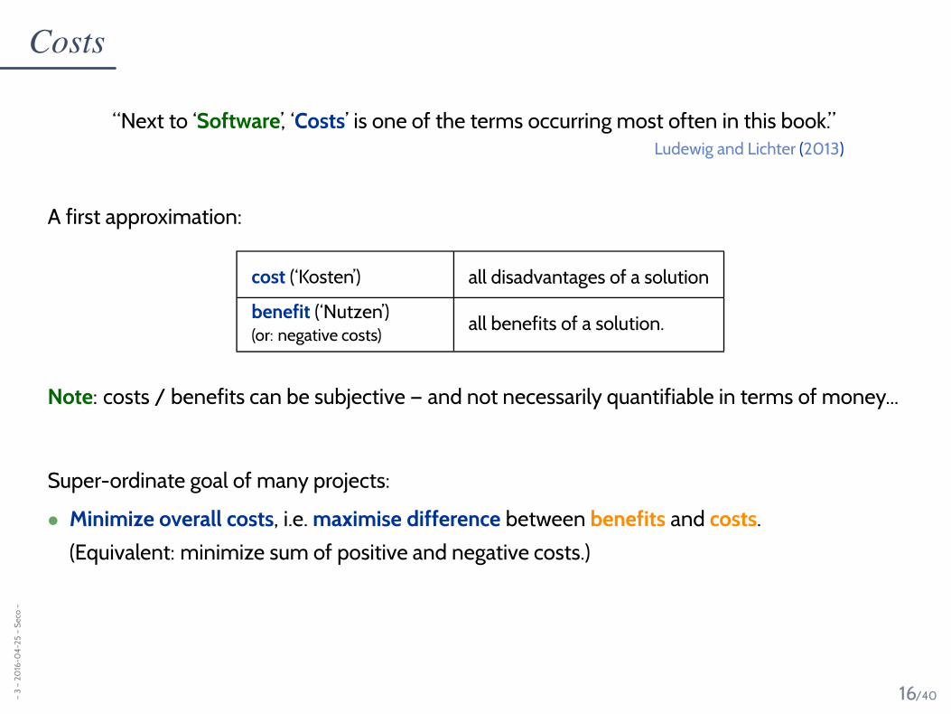
“Next to ‘Software’, ‘Costs’ is one of the terms occurring most often in this book.”Ludewig and Lichter (2013)
A first approximation:
cost (‘Kosten’) all disadvantages of a solution
benefit (‘Nutzen’)(or: negative costs)
all benefits of a solution.
Note: costs / benefits can be subjective — and not necessarily quantifiable in terms of money...
Super-ordinate goal of many projects:
• Minimize overall costs, i.e. maximise difference between benefits and costs.
(Equivalent: minimize sum of positive and negative costs.)
Costs vs. Benefits: A Closer Look–
3–
20
16-0
4-2
5–
Se
co–
17/40
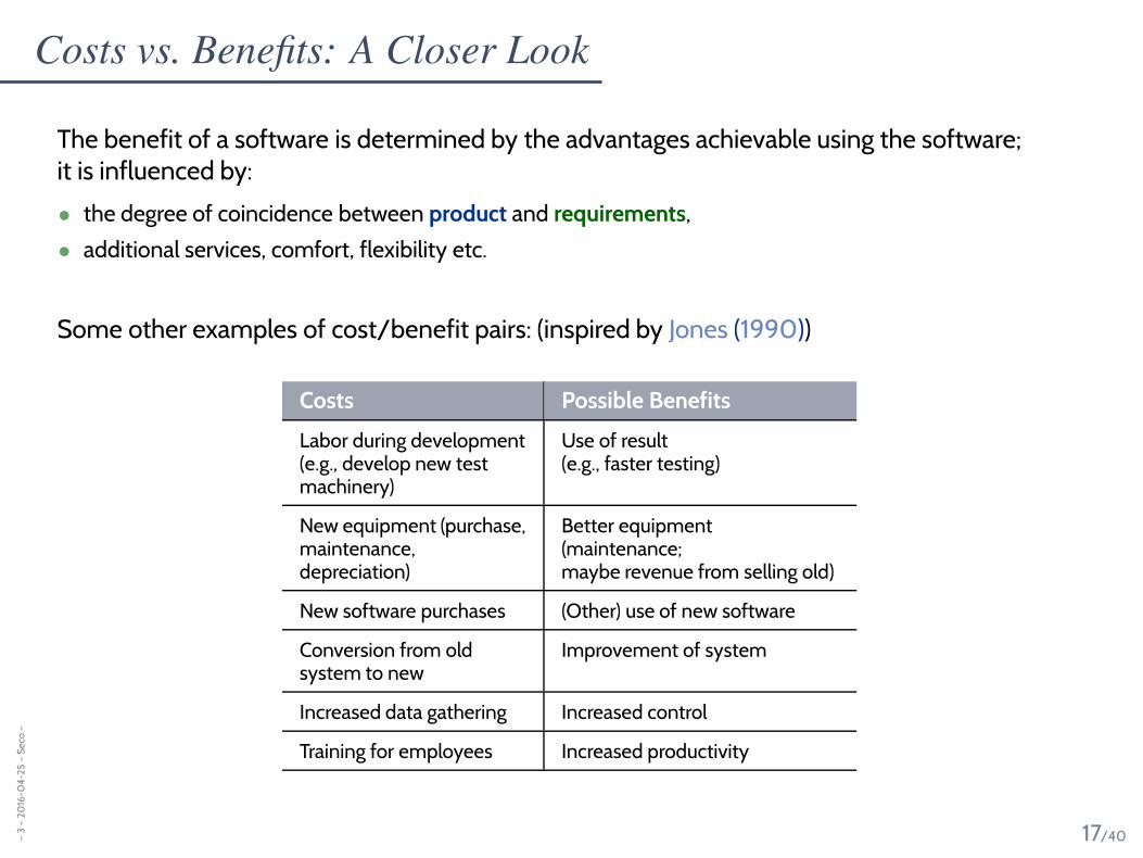
The benefit of a software is determined by the advantages achievable using the software;it is influenced by:
• the degree of coincidence between product and requirements,
• additional services, comfort, flexibility etc.
Some other examples of cost/benefit pairs: (inspired by Jones (1990))
Costs Possible Benefits
Labor during development(e.g., develop new testmachinery)
Use of result(e.g., faster testing)
New equipment (purchase,maintenance,depreciation)
Better equipment(maintenance;maybe revenue from selling old)
New software purchases (Other) use of new software
Conversion from oldsystem to new
Improvement of system
Increased data gathering Increased control
Training for employees Increased productivity
Costs: Economics in a Nutshell–
3–
20
16-0
4-2
5–
Se
co–
18/40
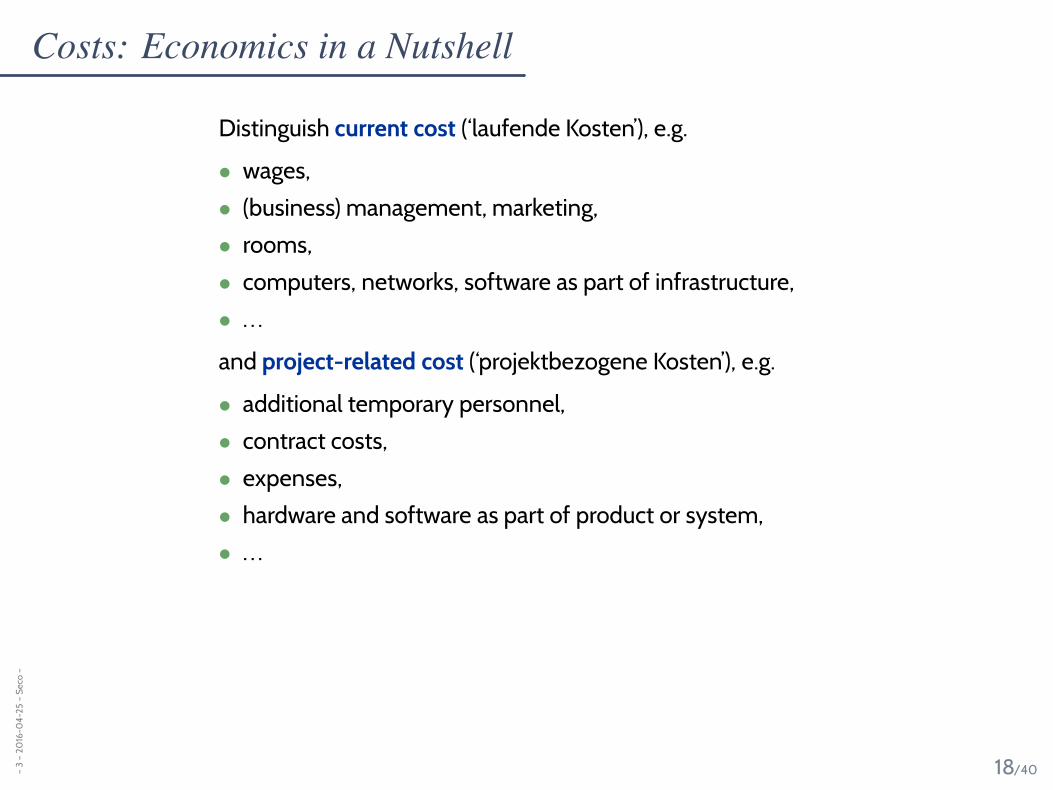
Distinguish current cost (‘laufende Kosten’), e.g.
• wages,
• (business) management, marketing,
• rooms,
• computers, networks, software as part of infrastructure,
• . . .
and project-related cost (‘projektbezogene Kosten’), e.g.
• additional temporary personnel,
• contract costs,
• expenses,
• hardware and software as part of product or system,
• . . .
westphal
Bleistift
westphal
Bleistift
westphal
Bleistift
westphal
Bleistift
westphal
Bleistift
Software Costs in a Narrower Sense–
3–
20
16-0
4-2
5–
Se
co–
19/40
software costs
net production quality costs
error preventioncosts
analyse-and-fixcosts
error costs
error localisationcosts
error removalcosts
error caused costs(in operation)
decreased benefit
maintenance(without quality)
quality assurance
during and after development Ludewig and Lichter (2013)
Software Engineering — the establishment and use of sound engineeringprinciples to obtain economically software that is reliable and works effi-ciently on real machines. F. L. Bauer (1971) co
mm
on
s.w
ikim
ed
ia.o
rg(C
C-b
y-s
a3
.0)
westphal
Bleistift
Discovering Fundamental Errors Late Can Be Expensive–
3–
20
16-0
4-2
5–
Se
co–
20/40
2
5
10
20
50
100
200
relative cost of an error
Analysis Design Coding Test &Integration
Acceptance& Operation
phase of errordetection
larger projects
smaller projects
Relative error costs over latency according to investigations at IBM, etc.
By (Boehm, 1979); Visualisation: Ludewig and Lichter (2013).
Cost Estimation
–3
–2
016
-04
-25
–m
ain
–
21/40
Why Estimate Cost?–
3–
20
16-0
4-2
5–
Se
stim
atio
n–
22/40
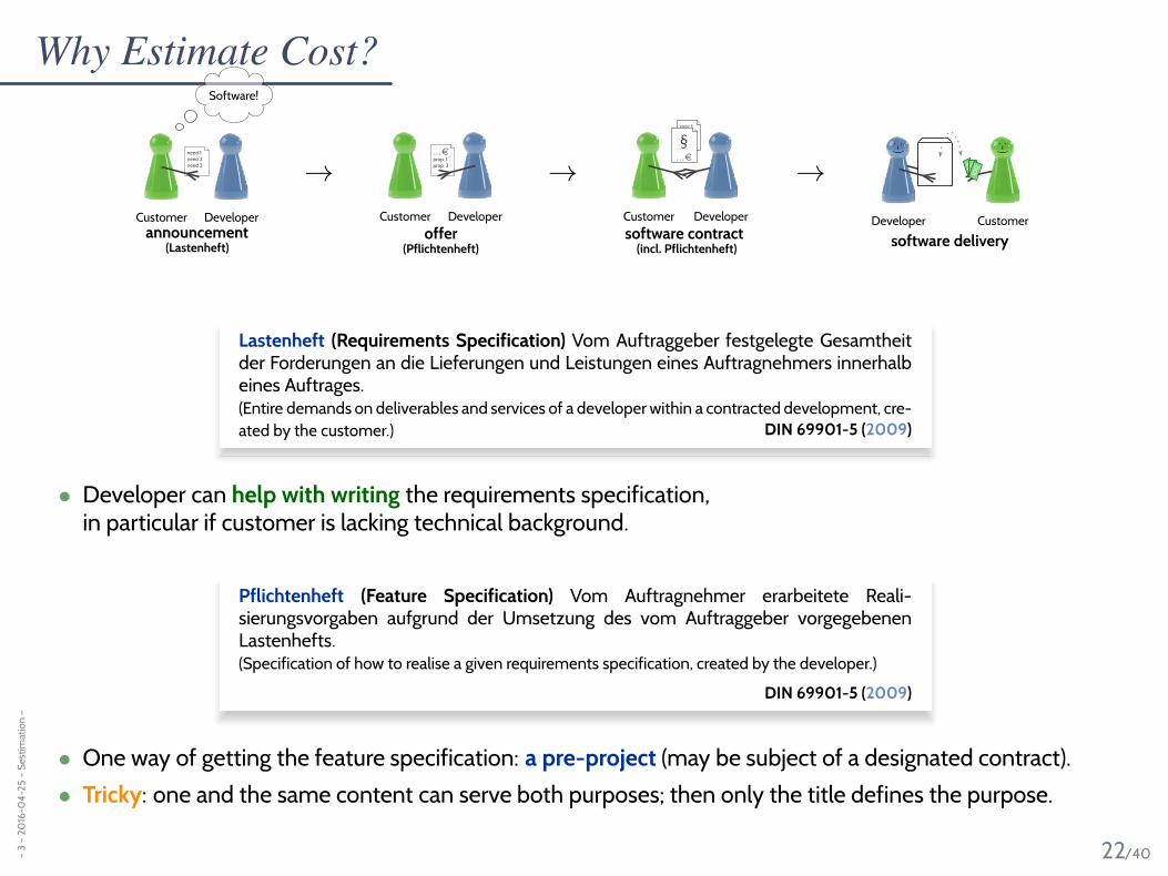
Software!
need 1need 2need 3. . .
Customer Developer
announcement(Lastenheft)
→
. . .eprop. 1prop. 2. . .
Customer Developer
offer(Pflichtenheft)
→
spec 1spec 2aspec 2b. . .§
. . .e
Customer Developer
software contract(incl. Pflichtenheft)
→
100
100
100
Developer Customer
software delivery
Lastenheft (Requirements Specification) Vom Auftraggeber festgelegte Gesamtheitder Forderungen an die Lieferungen und Leistungen eines Auftragnehmers innerhalbeines Auftrages.(Entire demands on deliverables and services of a developer within a contracted development, cre-
ated by the customer.) DIN 69901-5 (2009)
• Developer can help with writing the requirements specification,in particular if customer is lacking technical background.
Pflichtenheft (Feature Specification) Vom Auftragnehmer erarbeitete Reali-sierungsvorgaben aufgrund der Umsetzung des vom Auftraggeber vorgegebenenLastenhefts.(Specification of how to realise a given requirements specification, created by the developer.)
DIN 69901-5 (2009)
• One way of getting the feature specification: a pre-project (may be subject of a designated contract).
• Tricky: one and the same content can serve both purposes; then only the title defines the purpose.
westphal
Bleistift
The “Estimation Funnel”–
3–
20
16-0
4-2
5–
Se
stim
atio
n–
23/40
4×
2×
1×
0.5×
0.25×
effort estimated to realeffort (log. scale)
Pre-Project Analysis Design Coding & Test
t
Uncertainty with estimations (following (Boehm et al., 2000), p. 10).
Visualisation: Ludewig and Lichter (2013)
Plan–
3–
20
16-0
4-2
5–
Se
stim
atio
n–
24/40
• Cost Estimation
• “(Software) Economics in a Nutshell”
• Cost Estimation
• Expert’s Estimation
• The Delphi Method
• Algorithmic Estimation
• COCOMO
• Function Points
westphal
Bleistift
Expert’s Estimation
–3
–2
016
-04
-25
–S
est
imat
ion
–
25/40
Expert’s Estimation–
3–
20
16-0
4-2
5–
Se
stim
atio
n–
26/40
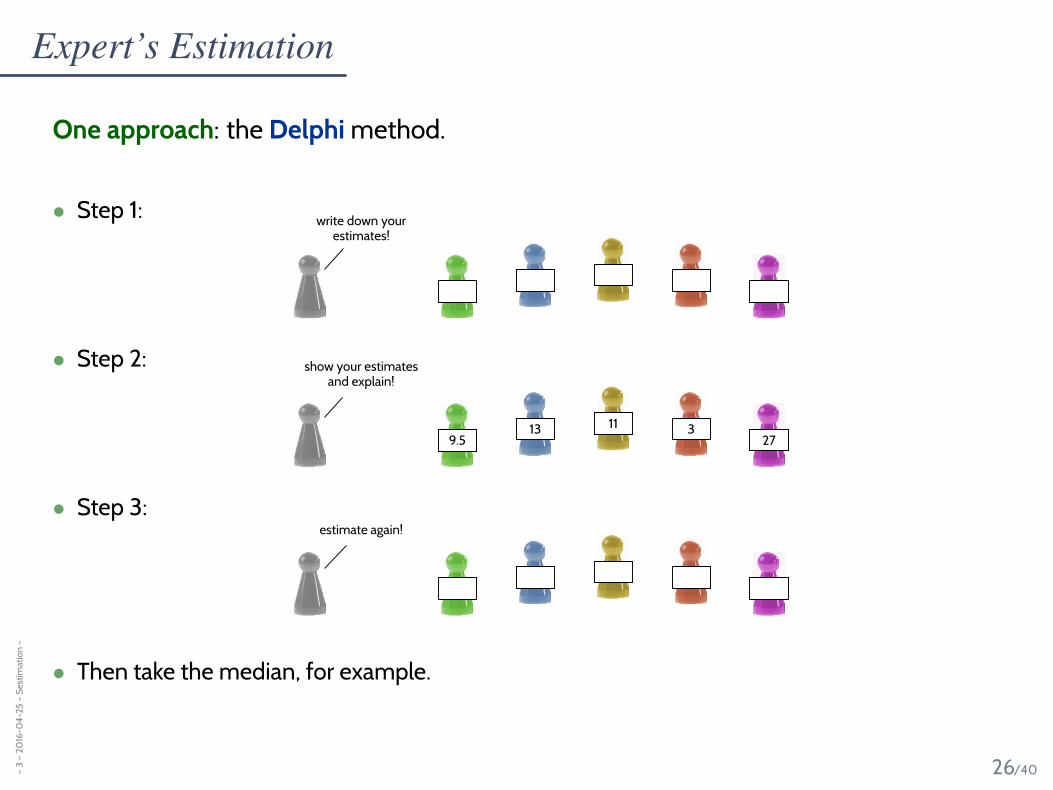
One approach: the Delphi method.
• Step 1:write down your
estimates!
• Step 2: show your estimatesand explain!
9.513 11 3
27
• Step 3:estimate again!
• Then take the median, for example.
Algorithmic Estimation
–3
–2
016
-04
-25
–S
est
imat
ion
–
27/40
Algorithmic Estimation: Principle–
3–
20
16-0
4-2
5–
Se
stim
atio
n–
28/40
P1 P2 P3 P4 P5
?
P6t
size /cost
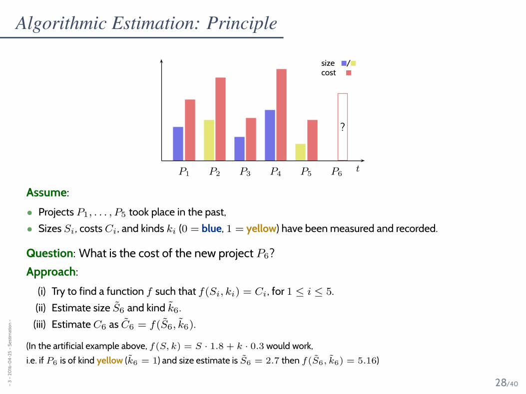
Assume:
• Projects P1, . . . , P5 took place in the past,
• Sizes Si , costs Ci, and kinds ki (0 = blue, 1 = yellow) have been measured and recorded.
Question: What is the cost of the new project P6?
Approach:
(i) Try to find a function f such that f(Si, ki) = Ci , for 1 ≤ i ≤ 5.
(ii) Estimate size S̃6 and kind k̃6.
(iii) Estimate C6 as C̃6 = f(S̃6, k̃6).
(In the artificial example above, f(S, k) = S · 1.8 + k · 0.3 would work,
i.e. if P6 is of kind yellow (k̃6 = 1) and size estimate is S̃6 = 2.7 then f(S̃6, k̃6) = 5.16)
westphal
Bleistift
westphal
Bleistift
Algorithmic Estimation: Principle–
3–
20
16-0
4-2
5–
Se
stim
atio
n–
28/40
P1 P2 P3 P4 P5
?
P6t
size /cost
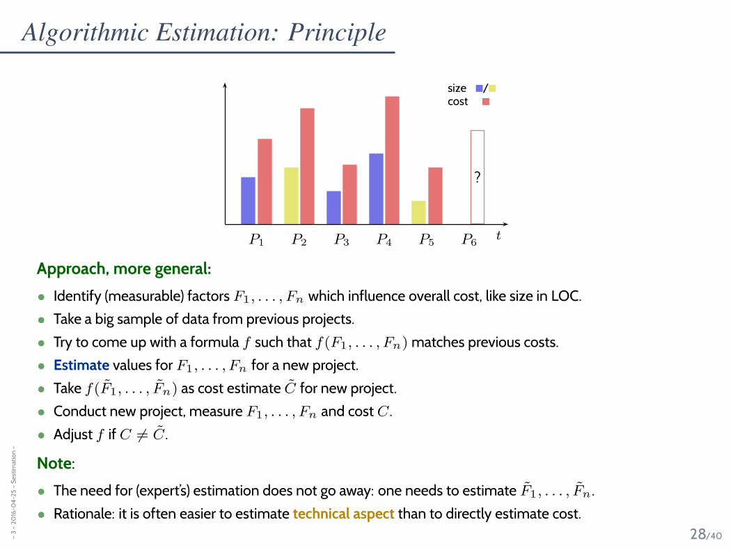
Approach, more general:
• Identify (measurable) factors F1, . . . , Fn which influence overall cost, like size in LOC.
• Take a big sample of data from previous projects.
• Try to come up with a formula f such that f(F1, . . . , Fn) matches previous costs.
• Estimate values for F1, . . . , Fn for a new project.
• Take f(F̃1, . . . , F̃n) as cost estimate C̃ for new project.
• Conduct new project, measure F1, . . . , Fn and cost C .
• Adjust f if C 6= C̃ .
westphal
Bleistift
Algorithmic Estimation: Principle–
3–
20
16-0
4-2
5–
Se
stim
atio
n–
28/40
P1 P2 P3 P4 P5
?
P6t
size /cost
Approach, more general:
• Identify (measurable) factors F1, . . . , Fn which influence overall cost, like size in LOC.
• Take a big sample of data from previous projects.
• Try to come up with a formula f such that f(F1, . . . , Fn) matches previous costs.
• Estimate values for F1, . . . , Fn for a new project.
• Take f(F̃1, . . . , F̃n) as cost estimate C̃ for new project.
• Conduct new project, measure F1, . . . , Fn and cost C .
• Adjust f if C 6= C̃ .
Note:
• The need for (expert’s) estimation does not go away: one needs to estimate F̃1, . . . , F̃n .
• Rationale: it is often easier to estimate technical aspect than to directly estimate cost.
westphal
Bleistift
westphal
Bleistift
Algorithmic Estimation: COCOMO–
3–
20
16-0
4-2
5–
Se
stim
atio
n–
29/40
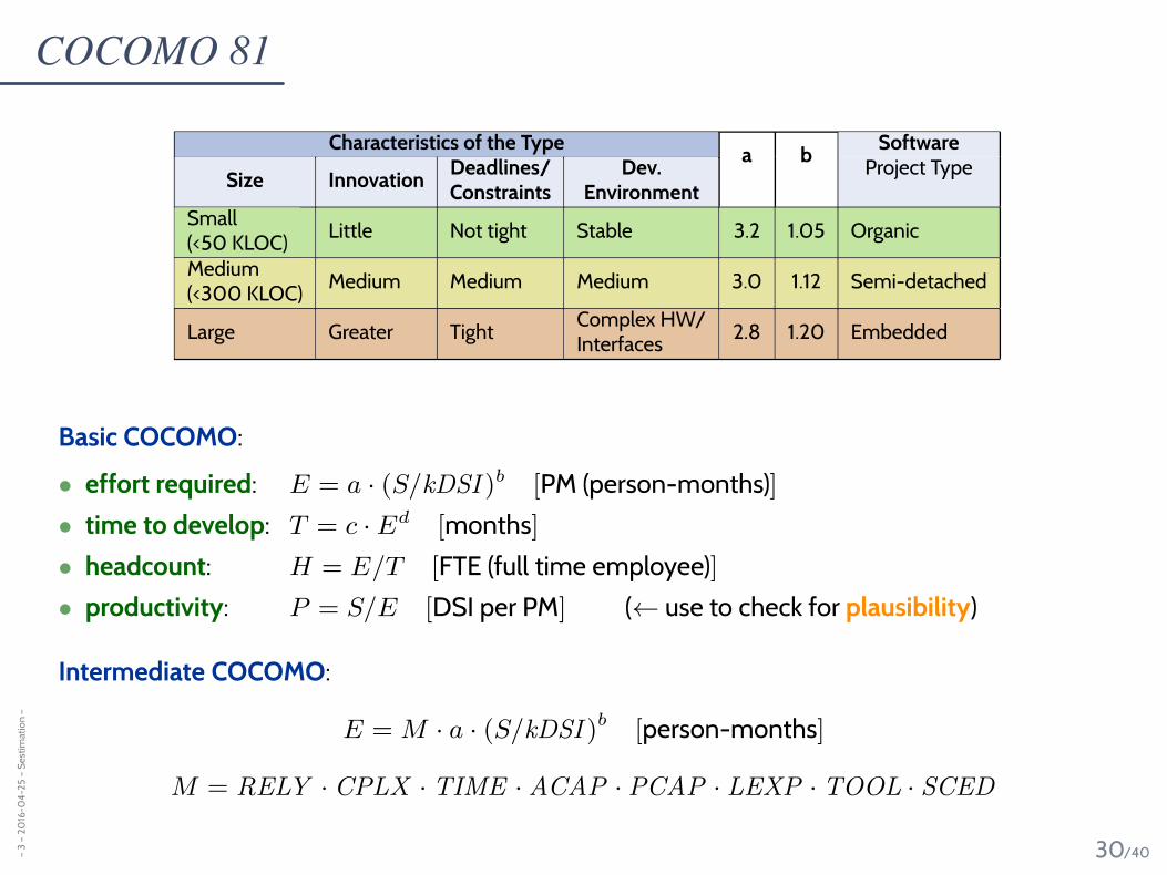
• Constructive Cost Model:Formulae which fit a huge set of archived project data (from the late 70’s).
LTEX experience with programming language(s) and tools
Project factors TOOL use of software tools
SITE degree of distributedness
SCED required development schedule
(also in COCOMO 81, new in COCOMO II)
Function Points
–3
–2
016
-04
-25
–S
est
imat
ion
–
35/40
Algorithmic Estimation: Function Points–
3–
20
16-0
4-2
5–
Se
stim
atio
n–
36/40
Complexity Sum
Type low medium high
input ·3 = ·4 = ·6 =
output ·4 = ·5 = ·7 =
query ·3 = ·4 = ·6 =
user data ·7 = ·10 = ·15 =
reference data ·5 = ·7 = ·10 =
Unadjusted function points UFP
Value adjustment factor VAF
Adjusted function points AFP = UFP · VAF
VAF = 0.65+1
100·
14∑
i=1
GSC i,
0 ≤ GSC i ≤ 5.
westphal
Bleistift
westphal
Bleistift
westphal
Bleistift
westphal
Bleistift
westphal
Bleistift
Algorithmic Estimation: Function Points–
3–
20
16-0
4-2
5–
Se
stim
atio
n–
36/40
Complexity Sum
Type low medium high
input ·3 = ·4 = ·6 =
output ·4 = ·5 = ·7 =
query ·3 = ·4 = ·6 =
user data ·7 = ·10 = ·15 =
reference data ·5 = ·7 = ·10 =
Unadjusted function points UFP
Value adjustment factor VAF
Adjusted function points AFP = UFP · VAF
IBM and VW curve for the conversion from AFPs to PM according to(Noth and Kretzschmar, 1984) and (Knöll and Busse, 1991).
VAF = 0.65+1
100·
14∑
i=1
GSC i,
0 ≤ GSC i ≤ 5.
westphal
Bleistift
Discussion–
3–
20
16-0
4-2
5–
Se
stim
atio
n–
37/40
Ludewig and Lichter (2013) says:
• Function Point approach used in practice,in particular for commercial software (business software?).
• COCOMO tends to overestimate in this domain;needs to be adjusted by corresponding factors.
In the end, it’s experience, experience, experience:
“Estimate, document, estimate better.” (Ludewig and Lichter, 2013)
Suggestion: start to explicate your experience now.
• Take notes on your projects(e.g., Softwarepraktikum, Bachelor Projekt, Master Bacherlor’s Thesis, Master Projekt, Master’s Thesis, . . . )
• timestamps, size of program created, number of errors found, number of pages written, . . .
• Try to identify factors: what hindered productivity, what boosted productivity, . . .
• Which detours and mistakes were avoidable in hindsight? How?
westphal
Bleistift
westphal
Bleistift
Tell Them What You’ve Told Them. . .–
3–
20
16-0
4-2
5–
Stt
wy
tt2
–
38/40
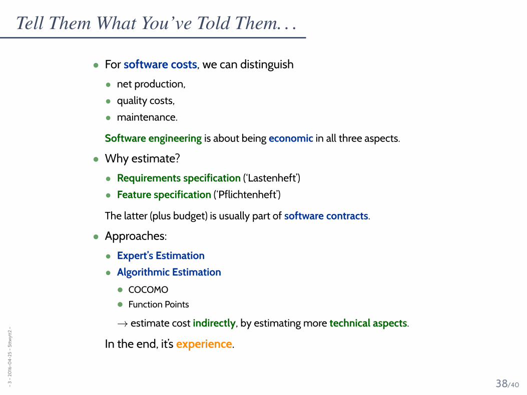
• For software costs, we can distinguish
• net production,
• quality costs,
• maintenance.
Software engineering is about being economic in all three aspects.
• Why estimate?
• Requirements specification (‘Lastenheft’)
• Feature specification (‘Pflichtenheft’)
The latter (plus budget) is usually part of software contracts.
• Approaches:
• Expert’s Estimation
• Algorithmic Estimation
• COCOMO
• Function Points
→ estimate cost indirectly, by estimating more technical aspects.
In the end, it’s experience.
westphal
Bleistift
References
–3
–2
016
-04
-25
–m
ain
–
39/40
References–
3–
20
16-0
4-2
5–
mai
n–
40/40
Basili, V. R. and Weiss, D. M. (1984). A methodology for collecting valid software engineering data. IEEETransactions of Software Engineering, 10(6):728–738.
Bauer, F. L. (1971). Software engineering. In IFIP Congress (1), pages 530–538.
Boehm, B. W. (1979). Guidelines for verifying and validating software requirements and design specifications. InEURO IFIP 79, pages 711–719. Elsevier North-Holland.
Boehm, B. W. (1981). Software Engineering Economics. Prentice-Hall.
Boehm, B. W., Horowitz, E., Madachy, R., Reifer, D., Clark, B. K., Steece, B., Brown, A. W., Chulani, S., and Abts, C.(2000). Software Cost Estimation with COCOMO II. Prentice-Hall.
Chidamber, S. R. and Kemerer, C. F. (1994). A metrics suite for object oriented design. IEEE Transactions onSoftware Engineering, 20(6):476–493.
DIN (2009). Projektmanagement; Projektmanagementsysteme. DIN 69901-5.
Jones, G. W. (1990). Software Engineering. John Wiley & Sons.
Kan, S. H. (2003). Metrics and models in Software Quality Engineering. Addison-Wesley, 2nd edition.
Knöll, H.-D. and Busse, J. (1991). Aufwandsschätzung von Software-Projekten in der Praxis: Methoden,Werkzeugeinsatz, Fallbeispiele. Number 8 in Reihe Angewandte Informatik. BI Wissenschaftsverlag.
Ludewig, J. and Lichter, H. (2013). Software Engineering. dpunkt.verlag, 3. edition.
Noth, T. and Kretzschmar, M. (1984). Aufwandsschätzung von DV-Projekten, Darstellung und Praxisvergleich derwichtigsten Verfahren. Springer-Verlag.