Lecture 30 Reciprocity Theorem Reciprocity theorem is one of the most important theorems in electromagnetics. With it we can develop physical intuition to ascertain if a certain design or experiment is right or wrong. It also tells us what is possible or impossible in the design of many systems. Reciprocity theorem is like “tit-for-tat” relationship in humans: Good-will is reciprocated with good will while ill-will is countered with ill-will. Both Confucius (551 BC–479 BC) and Jesus Christ (4 BC–AD 30) epoused the concept that, “Don’t do unto others that you don’t like others to do unto you.” But in electromagnetics, this beautiful relationship can be expressed precisely and succinctly using mathematics. We shall see how this is done. Figure 30.1: (Left) A depiction of Confucius from a stone fresco from the Western Han dynasty (202 BC–9 AD). The emphasis of the importance of “reciprocity” by Confucius Analects translated by D. Hinton [175]. (Right) A portrait of Jesus that is truer to its form. Jesus teaching from the New Testament says, “Do unto others as you would have them do unto you.” Luke 6:31 and Matthew 7:12 [176]. The subsequent portraits of these two sages are more humanly urbane. 327
Transcript
Lecture 30
Reciprocity Theorem
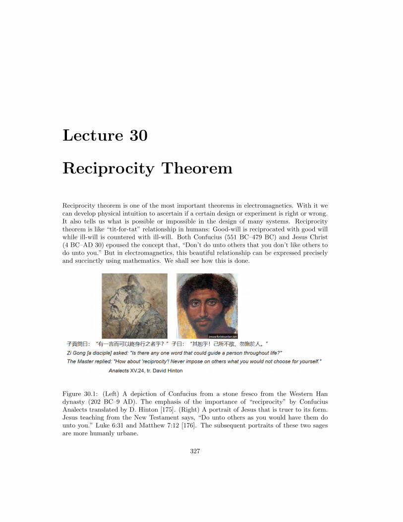
Reciprocity theorem is one of the most important theorems in electromagnetics. With it wecan develop physical intuition to ascertain if a certain design or experiment is right or wrong.It also tells us what is possible or impossible in the design of many systems. Reciprocitytheorem is like “tit-for-tat” relationship in humans: Good-will is reciprocated with good willwhile ill-will is countered with ill-will. Both Confucius (551 BC–479 BC) and Jesus Christ(4 BC–AD 30) epoused the concept that, “Don’t do unto others that you don’t like others todo unto you.” But in electromagnetics, this beautiful relationship can be expressed preciselyand succinctly using mathematics. We shall see how this is done.
Figure 30.1: (Left) A depiction of Confucius from a stone fresco from the Western Handynasty (202 BC–9 AD). The emphasis of the importance of “reciprocity” by ConfuciusAnalects translated by D. Hinton [175]. (Right) A portrait of Jesus that is truer to its form.Jesus teaching from the New Testament says, “Do unto others as you would have them dounto you.” Luke 6:31 and Matthew 7:12 [176]. The subsequent portraits of these two sagesare more humanly urbane.
327
328 Electromagnetic Field Theory
30.1 Mathematical Derivation
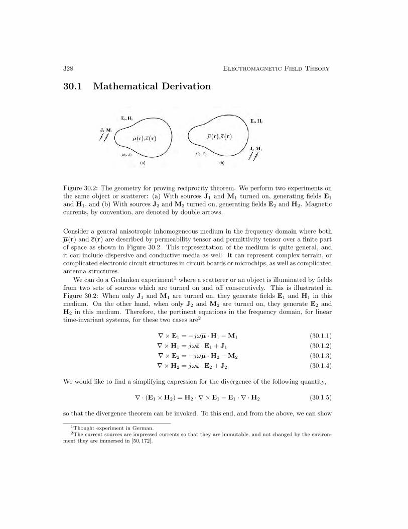
Figure 30.2: The geometry for proving reciprocity theorem. We perform two experiments onthe same object or scatterer: (a) With sources J1 and M1 turned on, generating fields E1
and H1, and (b) With sources J2 and M2 turned on, generating fields E2 and H2. Magneticcurrents, by convention, are denoted by double arrows.
Consider a general anisotropic inhomogeneous medium in the frequency domain where bothµ(r) and ε(r) are described by permeability tensor and permittivity tensor over a finite partof space as shown in Figure 30.2. This representation of the medium is quite general, andit can include dispersive and conductive media as well. It can represent complex terrain, orcomplicated electronic circuit structures in circuit boards or microchips, as well as complicatedantenna structures.
We can do a Gedanken experiment1 where a scatterer or an object is illuminated by fieldsfrom two sets of sources which are turned on and off consecutively. This is illustrated inFigure 30.2: When only J1 and M1 are turned on, they generate fields E1 and H1 in thismedium. On the other hand, when only J2 and M2 are turned on, they generate E2 andH2 in this medium. Therefore, the pertinent equations in the frequency domain, for lineartime-invariant systems, for these two cases are2
∇×E1 = −jωµ ·H1 −M1 (30.1.1)
∇×H1 = jωε ·E1 + J1 (30.1.2)
∇×E2 = −jωµ ·H2 −M2 (30.1.3)
∇×H2 = jωε ·E2 + J2 (30.1.4)
We would like to find a simplifying expression for the divergence of the following quantity,
∇ · (E1 ×H2) = H2 · ∇ ×E1 −E1 · ∇ ·H2 (30.1.5)
so that the divergence theorem can be invoked. To this end, and from the above, we can show
1Thought experiment in German.2The current sources are impressed currents so that they are immutable, and not changed by the environ-
ment they are immersed in [50,172].
Reciprocity Theorem 329
that (after left dot-multiply (30.1.1) with H2 and (30.1.4) with E1),
H2 · ∇ ×E1 = −jωH2 · µ ·H1 −H2 ·M1 (30.1.6)
E1 · ∇ ×H2 = jωE1 · ε ·E2 + E1 · J2 (30.1.7)
Then, using the above, and the following identity, we get the second equality in the followingexpression:
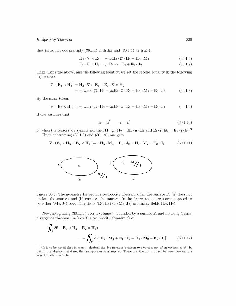
Figure 30.3: The geometry for proving reciprocity theorem when the surface S: (a) does notenclose the sources, and (b) encloses the sources. In the figure, the sources are supposed tobe either (M1,J1) producing fields (E1,H1) or (M2,J2) producing fields (E2,H2).
Now, integrating (30.1.11) over a volume V bounded by a surface S, and invoking Gauss’divergence theorem, we have the reciprocity theorem that
S
dS · (E1 ×H2 −E2 ×H1)
= −
V
dV [H2 ·M1 + E1 · J2 −H1 ·M2 −E2 · J1] (30.1.12)
3It is to be noted that in matrix algebra, the dot product between two vectors are often written as at · b,but in the physics literature, the transpose on a is implied. Therefore, the dot product between two vectorsis just written as a · b.
330 Electromagnetic Field Theory
When the volume V contains no sources (see Figure 30.3), the reciprocity theorem reduces to
S
dS · (E1 ×H2 −E2 ×H1) = 0 (30.1.13)
The above is also called Lorentz reciprocity theorem by some authors.4
Next, when the surface S contains all the sources (see Figure 30.3), then the right-handside of (30.1.12) will not be zero. On the other hand, when the surface S → ∞, E1 andH2 becomes spherical waves which can be approximated by plane waves sharing the same βvector. Moreover, under the plane-wave approximation, ωµ0H2 = β×E2, ωµ0H1 = β×E1,then
But β ·E2 = β ·E1 = 0 in the far field and the β vectors are parallel to each other. Therefore,the two terms on the left-hand side of (30.1.12) cancel each other, and it vanishes whenS →∞. (They cancel each other so that the remnant field vanishes faster than 1/r2. This isnecessary as the surface area S is growing larger and proportional to r2.)
As a result, when S →∞, (30.1.12) can be rewritten simply as
V
dV [E2 · J1 −H2 ·M1] =
V
dV [E1 · J2 −H1 ·M2] (30.1.16)
The inner product symbol is often used to rewrite the above as
〈E2,J1〉 − 〈H2,M1〉 = 〈E1,J2〉 − 〈H1,M2〉 (30.1.17)
where the inner product 〈A,B〉 =VdVA(r) ·B(r).
The above inner product is also called reaction, a concept introduced by Rumsey [177].The above is also called the Rumsey reaction theorem. Sometimes, the above is rewrittenmore succinctly and tersely as
〈2, 1〉 = 〈1, 2〉 (30.1.18)
where
〈2, 1〉 = 〈E2,J1〉 − 〈H2,M1〉 (30.1.19)
The concept of inner product or reaction can be thought of as a kind of “measurement”. Thereciprocity theorem can be stated as that the fields generated by sources 2 as “measured”by sources 1 is equal to fields generated by sources 1 as “measured” by sources 2. Thismeasurement concept is more lucid if we think of these sources as Hertzian dipoles.
4Harrington, Time-Harmonic Electric Field [50].
Reciprocity Theorem 331
30.2 Conditions for Reciprocity
It is seen that the above proof hinges on (30.1.10). In other words, the anisotropic mediumhas to be described by symmetric tensors. They include conductive media, but not gyrotropicmedia which is non-reciprocal. A ferrite biased by a magnetic field is often used in electroniccircuits, and it corresponds to a gyrotropic, non-reciprocal medium.5 Also, our startingequations (30.1.1) to (30.1.4) assume that the medium and the equations are linear timeinvariant so that Maxwell’s equations can be written down in the frequency domain easily.
30.3 Application to a Two-Port Network and CircuitTheory
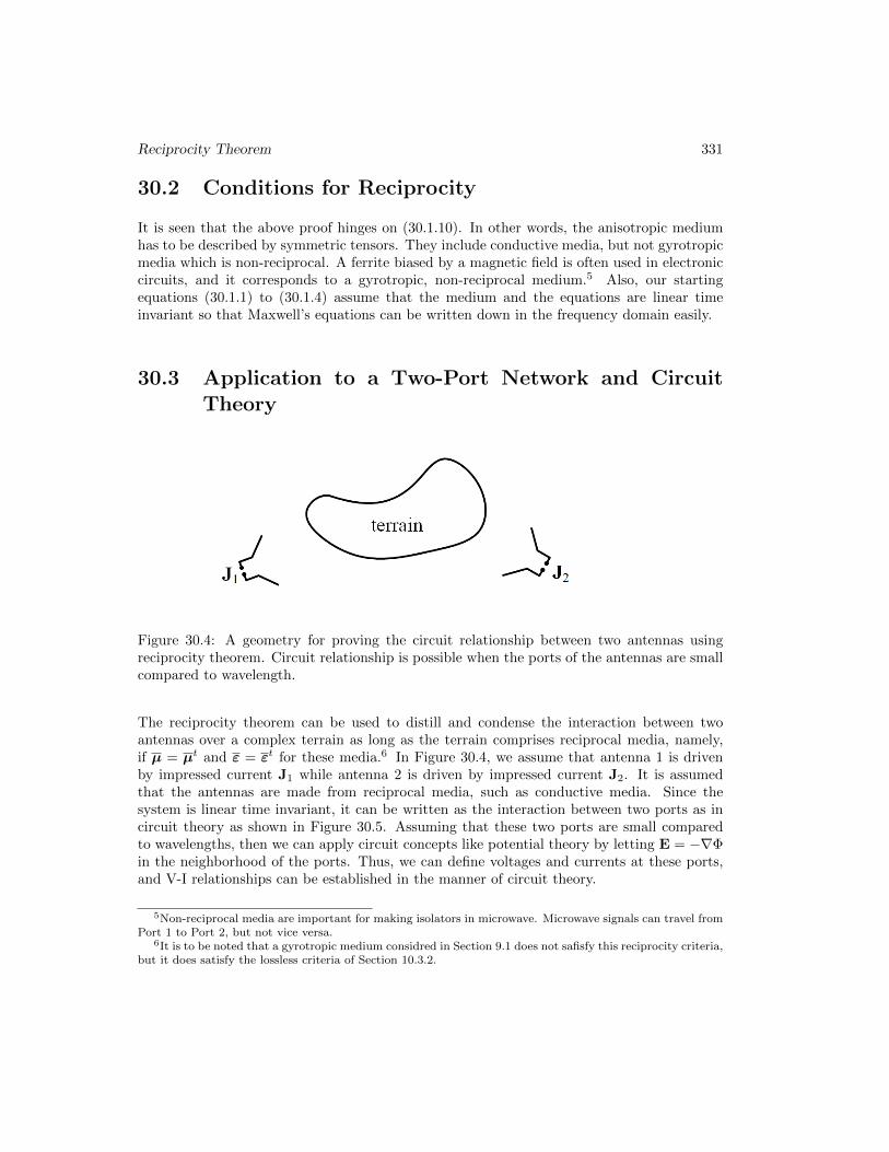
Figure 30.4: A geometry for proving the circuit relationship between two antennas usingreciprocity theorem. Circuit relationship is possible when the ports of the antennas are smallcompared to wavelength.
The reciprocity theorem can be used to distill and condense the interaction between twoantennas over a complex terrain as long as the terrain comprises reciprocal media, namely,if µ = µt and ε = εt for these media.6 In Figure 30.4, we assume that antenna 1 is drivenby impressed current J1 while antenna 2 is driven by impressed current J2. It is assumedthat the antennas are made from reciprocal media, such as conductive media. Since thesystem is linear time invariant, it can be written as the interaction between two ports as incircuit theory as shown in Figure 30.5. Assuming that these two ports are small comparedto wavelengths, then we can apply circuit concepts like potential theory by letting E = −∇Φin the neighborhood of the ports. Thus, we can define voltages and currents at these ports,and V-I relationships can be established in the manner of circuit theory.
5Non-reciprocal media are important for making isolators in microwave. Microwave signals can travel fromPort 1 to Port 2, but not vice versa.
6It is to be noted that a gyrotropic medium considred in Section 9.1 does not safisfy this reciprocity criteria,but it does satisfy the lossless criteria of Section 10.3.2.
332 Electromagnetic Field Theory
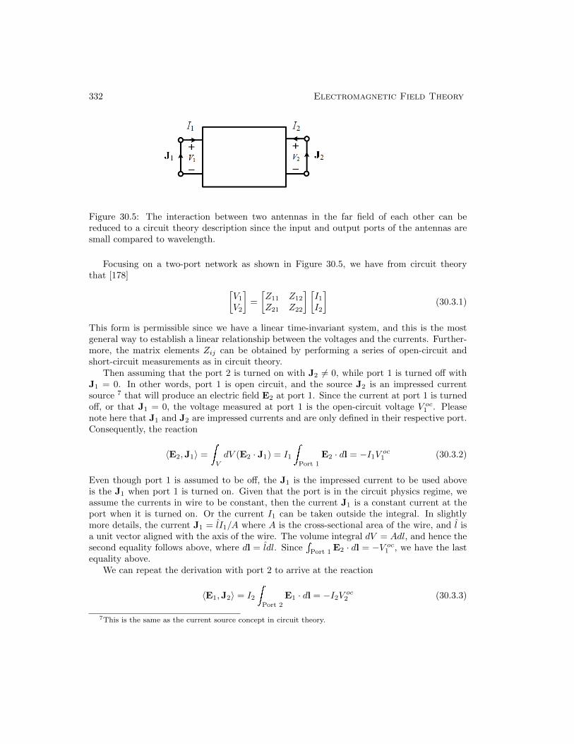
Figure 30.5: The interaction between two antennas in the far field of each other can bereduced to a circuit theory description since the input and output ports of the antennas aresmall compared to wavelength.
Focusing on a two-port network as shown in Figure 30.5, we have from circuit theorythat [178] [
V1
V2
]=
[Z11 Z12
Z21 Z22
] [I1I2
](30.3.1)
This form is permissible since we have a linear time-invariant system, and this is the mostgeneral way to establish a linear relationship between the voltages and the currents. Further-more, the matrix elements Zij can be obtained by performing a series of open-circuit andshort-circuit measurements as in circuit theory.
Then assuming that the port 2 is turned on with J2 6= 0, while port 1 is turned off withJ1 = 0. In other words, port 1 is open circuit, and the source J2 is an impressed currentsource 7 that will produce an electric field E2 at port 1. Since the current at port 1 is turnedoff, or that J1 = 0, the voltage measured at port 1 is the open-circuit voltage V oc1 . Pleasenote here that J1 and J2 are impressed currents and are only defined in their respective port.Consequently, the reaction
〈E2,J1〉 =
V
dV (E2 · J1) = I1
Port 1
E2 · dl = −I1V oc1 (30.3.2)
Even though port 1 is assumed to be off, the J1 is the impressed current to be used aboveis the J1 when port 1 is turned on. Given that the port is in the circuit physics regime, weassume the currents in wire to be constant, then the current J1 is a constant current at theport when it is turned on. Or the current I1 can be taken outside the integral. In slightlymore details, the current J1 = lI1/A where A is the cross-sectional area of the wire, and l isa unit vector aligned with the axis of the wire. The volume integral dV = Adl, and hence thesecond equality follows above, where dl = ldl. Since
Port 1
E2 · dl = −V oc1 , we have the lastequality above.
We can repeat the derivation with port 2 to arrive at the reaction
〈E1,J2〉 = I2
Port 2
E1 · dl = −I2V oc2 (30.3.3)
7This is the same as the current source concept in circuit theory.
Reciprocity Theorem 333
Reciprocity requires these two reactions to be equal, and hence,
I1Voc1 = I2V
oc2
But from (30.3.1), we can set the pertinent currents to zero to find these open circuit voltages.Therefore, V oc1 = Z12I2, V oc2 = Z21I1. Since I1V
oc1 = I2V
oc2 by the reaction concept or by
reciprocity, then Z12 = Z21. The above analysis can be easily generalized to an N -portnetwork.
The simplicity of the above belies its importance. The above shows that the reciprocityconcept in circuit theory is a special case of reciprocity theorem for electromagnetic theory.The terrain can also be replaced by complex circuits as in a circuit board, as long as thematerials in the terrain or circuit board are reciprocal, linear and time invariant. For instance,the complex terrain can also be replaced by complex antenna structures. It is to be notedthat even when the transmit and receive antennas area miles apart, as long as the transmitand receive ports of the linear system can be characterized by a linear relation expounded by(30.3.1), and the ports small enough compared to wavelength so that circuit theory prevails,we can apply the above analysis! This relation that Z12 = Z21 is true as long as the mediumtraversed by the fields is a reciprocal medium.
Before we conclude this section, it is to be mentioned that some researchers advocate theuse of circuit theory to describe electromagnetic theory. Such is the case in the transmissionline matrix (TLM) method [179], and the partial element equivalence circuit (PEEC) method[180]. Circuit theory is so simple that many people fall in love with it!
30.4 Voltage Sources in Electromagnetics
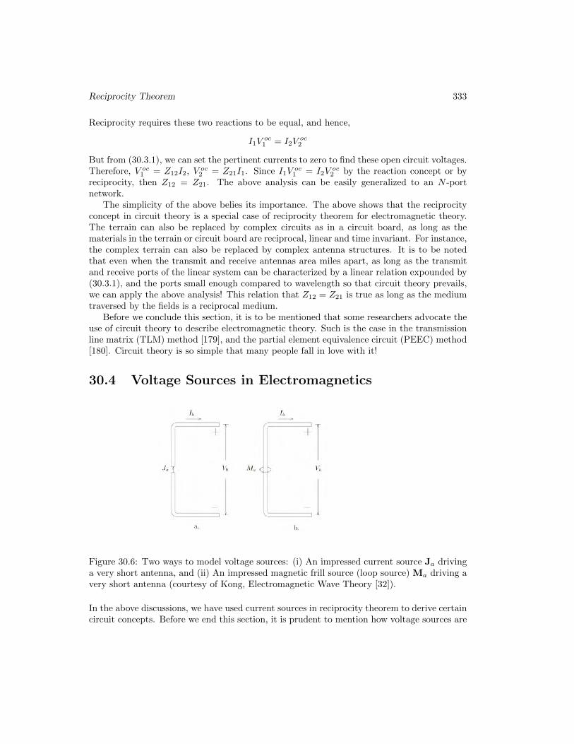
Figure 30.6: Two ways to model voltage sources: (i) An impressed current source Ja drivinga very short antenna, and (ii) An impressed magnetic frill source (loop source) Ma driving avery short antenna (courtesy of Kong, Electromagnetic Wave Theory [32]).
In the above discussions, we have used current sources in reciprocity theorem to derive certaincircuit concepts. Before we end this section, it is prudent to mention how voltage sources are
334 Electromagnetic Field Theory
modeled in electromagnetic theory. The use of the impressed currents so that circuit conceptscan be applied is shown in Figure 30.6. The antenna in (a) is driven by a current source.But a magnetic current can be used as a voltage source in circuit theory as shown by Figure30.6b. By using duality concept, an electric field has to curl around a magnetic current justin Ampere’s law where magnetic field curls around an electric current. This electric field willcause a voltage drop between the metal above and below the magnetic current loop makingit behave like a voltage source.8
30.5 Hind Sight
The proof of reciprocity theorem for Maxwell’s equations is very deeply related to the sym-metry of the operator involved. We can see this from linear algebra. Given a matrix equationdriven by two different sources b1 and b2 with solutions x1 and x2, they can be writtensuccinctly as
A · x1 = b1 (30.5.1)
A · x2 = b2 (30.5.2)
We can left dot multiply the first equation with x2 and do the same with the second equationwith x1 to arrive at
xt2 ·A · x1 = xt2 · b1 (30.5.3)
xt1 ·A · x2 = xt1 · b2 (30.5.4)
If A is symmetric, the left-hand side of both equations are equal to each other.9 Therefore,we can equate their right-hand side to arrive at
xt2 · b1 = xt1 · b2 (30.5.5)
The above is analogous to the statement of the reciprocity theorem which is
〈E2,J1〉 = 〈E1,J2〉 (30.5.6)
where the reaction inner product, as mentioned before, is 〈Ei,Jj〉 =V
Ei(r)·Jj(r). The innerproduct in linear algebra is that of dot product in matrix theory, but the inner product forreciprocity theorem is that for infinite dimensional spaces.10 So if the operators in Maxwell’sequations are symmetrical, then reciprocity theorem applies.
8More can be found in Jordain and Balmain, Electromagnetic Waves and Radiation Systems [54].9This can be easily proven by taking the transpose of a scalar, and taking the transpose of the product of
matrices.10Such spaces are called Hilbert space.
Reciprocity Theorem 335
30.6 Transmit and Receive Patterns of an Antennna
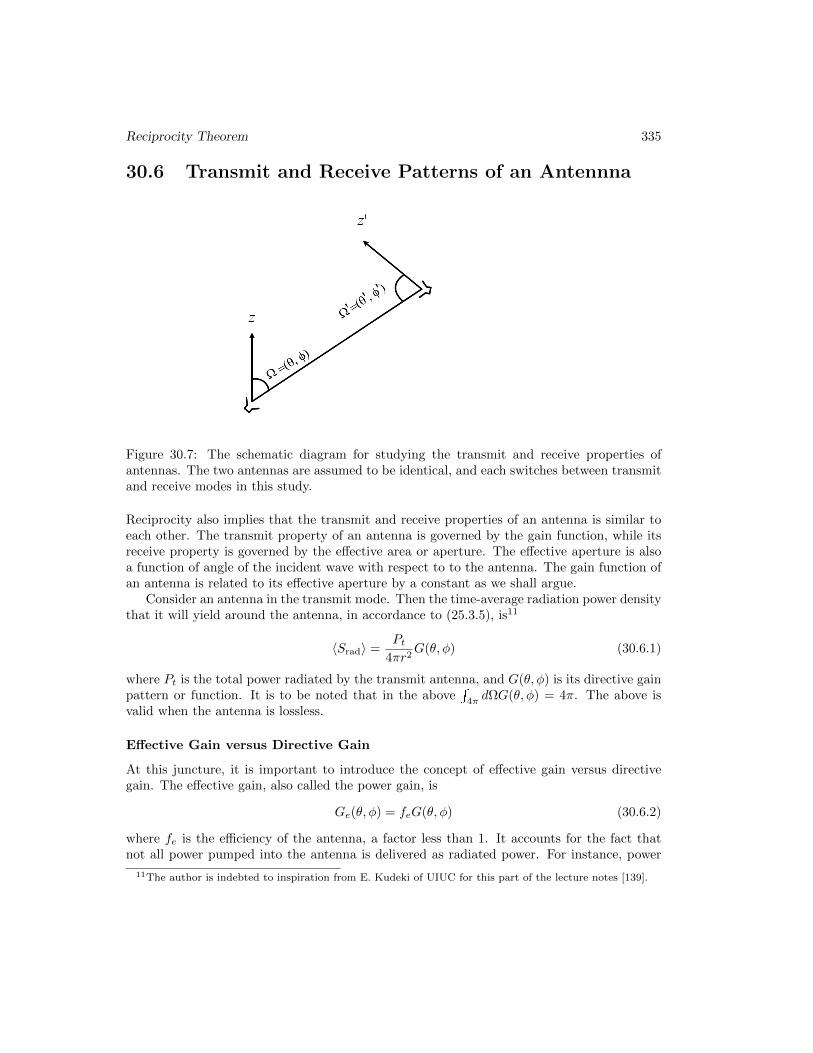
Figure 30.7: The schematic diagram for studying the transmit and receive properties ofantennas. The two antennas are assumed to be identical, and each switches between transmitand receive modes in this study.
Reciprocity also implies that the transmit and receive properties of an antenna is similar toeach other. The transmit property of an antenna is governed by the gain function, while itsreceive property is governed by the effective area or aperture. The effective aperture is alsoa function of angle of the incident wave with respect to to the antenna. The gain function ofan antenna is related to its effective aperture by a constant as we shall argue.
Consider an antenna in the transmit mode. Then the time-average radiation power densitythat it will yield around the antenna, in accordance to (25.3.5), is11
〈Srad〉 =Pt
4πr2G(θ, φ) (30.6.1)
where Pt is the total power radiated by the transmit antenna, and G(θ, φ) is its directive gainpattern or function. It is to be noted that in the above
4πdΩG(θ, φ) = 4π. The above is
valid when the antenna is lossless.
Effective Gain versus Directive Gain
At this juncture, it is important to introduce the concept of effective gain versus directivegain. The effective gain, also called the power gain, is
Ge(θ, φ) = feG(θ, φ) (30.6.2)
where fe is the efficiency of the antenna, a factor less than 1. It accounts for the fact thatnot all power pumped into the antenna is delivered as radiated power. For instance, power
11The author is indebted to inspiration from E. Kudeki of UIUC for this part of the lecture notes [139].
336 Electromagnetic Field Theory
can be lost in the circuits and mismatch of the antenna. Therefore, the correct formula theradiated power density is
〈Srad〉 =Pt
4πr2Ge(θ, φ) = fe
Pt4πr2
G(θ, φ) (30.6.3)
This radiated power resembles that of a plane wave when one is far away from the trans-mitter. Thus if a receive antenna is placed in the far-field of the transmit antenna, it willsee this power density as coming from a plane wave. Thus the receive antenna will see anincident power density as
〈Sinc〉 = 〈Srad〉 =Pt
4πr2Ge(θ, φ) (30.6.4)
Effective Aperture
The effective area or the aperture of a receive antenna is used to characterize its receiveproperty. The power received by such an antenna is then, by using the concept of effectiveaperture expounded in (26.1.23)
Pr = 〈Sinc〉Ae(θ′, φ′) (30.6.5)
where (θ′, φ′) are the angles at which the plane wave is incident upon the receiving antenna(see Figure 30.7). Combining the above formulas (30.6.4) and (30.6.5), we have
Pr =Pt
4πr2Ge(θ, φ)Ae(θ
′, φ′) (30.6.6)
Now assuming that the transmit and receive antennas are identical. Next, we swap theirroles of transmit and receive, and also the circuitries involved in driving the transmit andreceive antennas. Then,
Pr =Pt
4πr2Ge(θ
′, φ′)Ae(θ, φ) (30.6.7)
We also assume that the receive antenna, that now acts as the transmit antenna is transmittingin the (θ′, φ′) direction. Moreover, the transmit antenna, that now acts as the receive antennais receiving in the (θ, φ) direction (see Figure 30.7).
By reciprocity, these two powers are the same, because Z12 = Z21. Furthermore, sincethese two antennas are identical, Z11 = Z22. So by swapping the transmit and receiveelectronics, the power transmitted and received will not change. A simple transmit-receivecircuit diagram is shown in Figure 30.8
Reciprocity Theorem 337
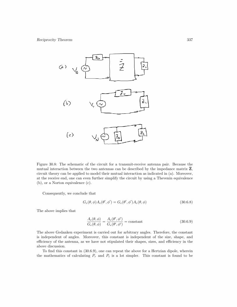
Figure 30.8: The schematic of the circuit for a transmit-receive antenna pair. Because themutual interaction between the two antennas can be described by the impedance matrix Z,circuit theory can be applied to model their mutual interaction as indicated in (a). Moreover,at the receive end, one can even further simplify the circuit by using a Thevenin equivalence(b), or a Norton equivalence (c).
Consequently, we conclude that
Ge(θ, φ)Ae(θ′, φ′) = Ge(θ
′, φ′)Ae(θ, φ) (30.6.8)
The above implies that
Ae(θ, φ)
Ge(θ, φ)=Ae(θ
′, φ′)
Ge(θ′, φ′)= constant (30.6.9)
The above Gedanken experiment is carried out for arbitrary angles. Therefore, the constantis independent of angles. Moreover, this constant is independent of the size, shape, andefficiency of the antenna, as we have not stipulated their shapes, sizes, and efficiency in theabove discussion.
To find this constant in (30.6.9), one can repeat the above for a Hertzian dipole, whereinthe mathematics of calculating Pr and Pt is a lot simpler. This constant is found to be
338 Electromagnetic Field Theory
λ2/(4π).12 Therefore, an interesting relationship between the effective aperture (or area) andthe directive gain function is that
Ae(θ, φ) =λ2
4πGe(θ, φ) (30.6.10)
One amusing point about the above formula is that the effective aperture, say of a Hertziandipole, becomes very large when the frequency is low, or the wavelength is very long. Ofcourse, this cannot be physically true, and I will let you meditate on this paradox and museover this point.
12See Kong [32][p. 700]. The derivation is for 100% efficient antenna. A thermal equilibrium argument isused in [139] and Wikipedia [140] as well.


![5 different superposition principles with/without test ...vixra.org/pdf/1811.0396v2.pdfcorrelation reciprocity theorem[7]. It can be proven that the cross correlation reciprocity theorem](https://static.documents.pub/doc/80x56/5ea307e43ad85b64472c4bb0/5-different-superposition-principles-withwithout-test-vixraorgpdf1811-correlation.jpg)


![BMS COLLEGE OF ENGINEERING, BANGALORE Syllabus 2009-12.pdf · Superposition, Reciprocity, Millman’s Thevinin’s and Norton’s theorems, Maximum Power transfer theorem. [12 Hours]](https://static.documents.pub/doc/80x56/5ebb32f790d45c1c153de3ec/bms-college-of-engineering-bangalore-syllabus-2009-12pdf-superposition-reciprocity.jpg)


