39
Lecture 3.2 Chapter 7 Firms in Perfectly Competitive Markets
| Date post: | 11-Dec-2015 |
| Category: |
Documents |
| Upload: | hassan-khan |
| View: | 217 times |
| Download: | 0 times |

Lecture 3.2 Chapter 7
Firms in Perfectly Competitive Markets
1. Explain what a perfectly competitive market is and why a perfect competitor faces a horizontal demand curve.
2. Explain how a firm maximises profits in a perfectly competitive market.
3. Use graphs to show a firm’s profit or loss.
4. Explain why firms may shut down temporarily.
5. Explain how entry and exit ensure that firms earn zero economic profit in the long run.
6. Explain how perfect competition leads to economic efficiency.
Learning Objectives
2 Copyright © 2013 Pearson Australia (a division of Pearson Australia Group Pty Ltd) – 9781442558069/Hubbard and O'Brien/Essentials of Economics/2e
Market structures
Economists group industries into four market structures:
Perfect competition
Monopolistic competition
Oligopoly
Monopoly
3 Copyright © 2013 Pearson Australia (a division of Pearson Australia Group Pty Ltd) – 9781442558069/Hubbard and O'Brien/Essentials of Economics/2e

Characteristic Perfect competition
Monopolistic competition
Oligopoly Monopoly
Number of firms
Many Many Few One
Type of product
Identical Differentiated Identical or differentiated
Unique
Ease of entry High High Low Entry blocked
Examples of industries
– Apples
– Wheat
– Selling DVDs
– Restaurants
– Banking– Manufacturing cars
– Letter delivery– Tap water
Copyright © 2013 Pearson Australia (a division of Pearson Australia Group Pty Ltd) – 9781442558069/Hubbard and O'Brien/Essentials of Economics/2e 4
The four market structures

Perfectly competitive markets
The conditions that make a market perfectly competitive are:
1. There are many buyers and sellers, all of whom are small relative to the market.
2. All firms sell identical products.
3. There are no barriers to new firms entering the market or to existing firms leaving the market.
5 Copyright © 2013 Pearson Australia (a division of Pearson Australia Group Pty Ltd) – 9781442558069/Hubbard and O'Brien/Essentials of Economics/2e
A perfectly competitive firm cannot affect the market price
Price taker: A buyer or seller that is unable to affect the market price.
The demand curve for a price taker is horizontal, or perfectly elastic.
6 Copyright © 2013 Pearson Australia (a division of Pearson Australia Group Pty Ltd) – 9781442558069/Hubbard and O'Brien/Essentials of Economics/2e
Perfectly competitive markets

Profit: Total revenue (TR) minus total cost (TC).
Profit = TR - TC
How a firm maximises profit in a perfectly competitive market
7 Copyright © 2013 Pearson Australia (a division of Pearson Australia Group Pty Ltd) – 9781442558069/Hubbard and O'Brien/Essentials of Economics/2e

(b) Demand for an individual farmer’s oats
0
(a) Market for oats
Quantity of oats (bushels per year)
Supply of oats
Demand for oats
$4
Demand for Farmer Jones’ oats
2. …which must be accepted by Farmer Jones and every other seller of oats.
80 000 000
Price of oats (dollars per bushel)
Price of oats (dollars per bushel)
Quantity of oats (bushels per year)
0 7500
$4
1. The intersection of market supply and market demand determines the equilibrium price of oats...
8 Copyright © 2013 Pearson Australia (a division of Pearson Australia Group Pty Ltd) – 9781442558069/Hubbard and O'Brien/Essentials of Economics/2e
Market demand and individual firm demand: Figure 7.2
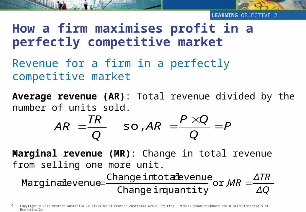
Revenue for a firm in a perfectly competitive market
Average revenue (AR): Total revenue divided by the number of units sold.
Marginal revenue (MR): Change in total revenue from selling one more unit.
Q
TRAR P
Q
QPAR
so,
or, ΔQ
ΔTRMR
quantity in Change
revenue total in Change revenue Marginal
Copyright © 2013 Pearson Australia (a division of Pearson Australia Group Pty Ltd) – 9781442558069/Hubbard and O'Brien/Essentials of Economics/2e 9
LEARNING OBJECTIVE 2
How a firm maximises profit in a perfectly competitive market
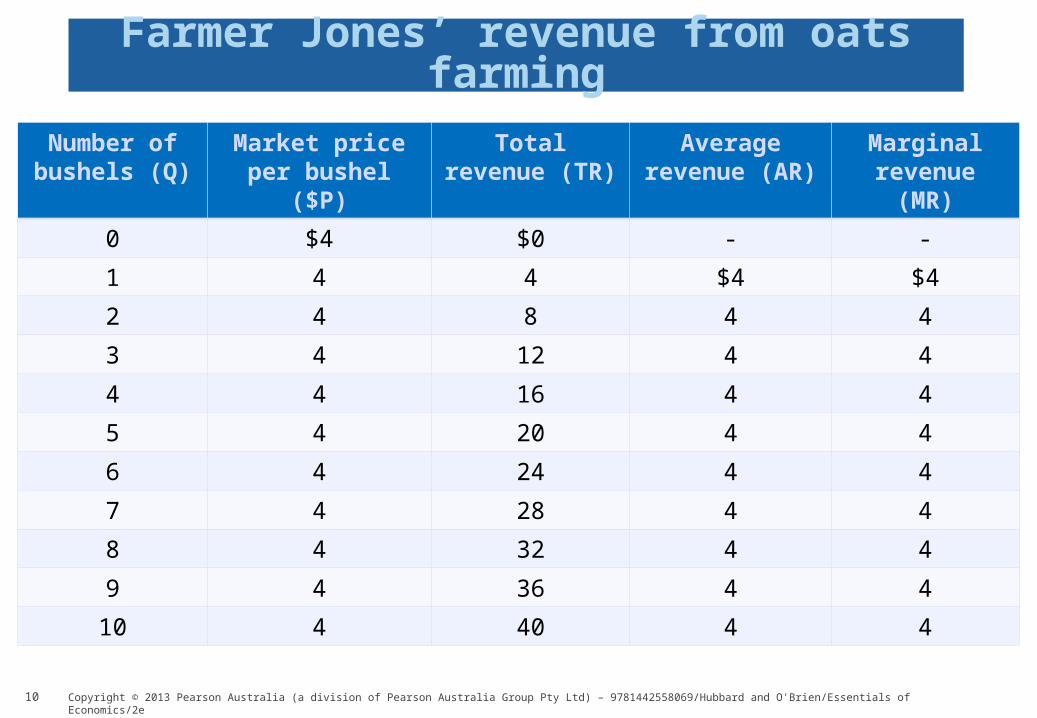
Number of bushels (Q)
Market price per bushel ($P)
Total revenue (TR)
Average revenue (AR)
Marginal revenue (MR)
0 $4 $0 - -
1 4 4 $4 $4
2 4 8 4 4
3 4 12 4 4
4 4 16 4 4
5 4 20 4 4
6 4 24 4 4
7 4 28 4 4
8 4 32 4 4
9 4 36 4 4
10 4 40 4 4
Copyright © 2013 Pearson Australia (a division of Pearson Australia Group Pty Ltd) – 9781442558069/Hubbard and O'Brien/Essentials of Economics/2e 10
Farmer Jones’ revenue from oats farming
Determining the profit-maximising level of output
Since producers in a perfectly competitive market can sell as much produce as they wish to at the same constant price:
Average revenue (AR) = Marginal revenue (MR)
Price = AR = MR
Copyright © 2013 Pearson Australia (a division of Pearson Australia Group Pty Ltd) – 9781442558069/Hubbard and O'Brien/Essentials of Economics/2e 11
How a firm maximises profit in a perfectly competitive market
Determining the profit-maximising level of output, cont.
The profit-maximising level of output is where the difference between total revenue and total cost is the greatest.
The profit-maximising level of output is also where marginal revenue equals marginal cost, or MR = MC.
Copyright © 2013 Pearson Australia (a division of Pearson Australia Group Pty Ltd) – 9781442558069/Hubbard and O'Brien/Essentials of Economics/2e 12
How a firm maximises profit in a perfectly competitive market
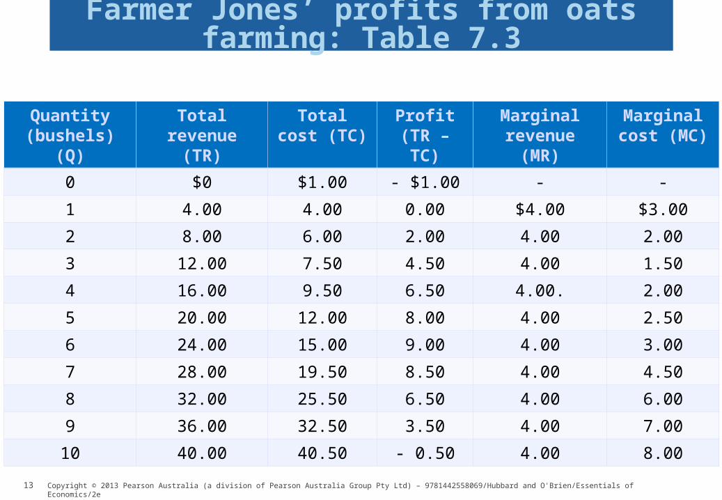
Quantity (bushels)(Q)
Total revenue (TR)
Total cost (TC)
Profit (TR – TC)
Marginal revenue (MR)
Marginal cost (MC)
0 $0 $1.00 - $1.00 - -
1 4.00 4.00 0.00 $4.00 $3.00
2 8.00 6.00 2.00 4.00 2.00
3 12.00 7.50 4.50 4.00 1.50
4 16.00 9.50 6.50 4.00. 2.00
5 20.00 12.00 8.00 4.00 2.50
6 24.00 15.00 9.00 4.00 3.00
7 28.00 19.50 8.50 4.00 4.50
8 32.00 25.50 6.50 4.00 6.00
9 36.00 32.50 3.50 4.00 7.00
10 40.00 40.50 - 0.50 4.00 8.00
Copyright © 2013 Pearson Australia (a division of Pearson Australia Group Pty Ltd) – 9781442558069/Hubbard and O'Brien/Essentials of Economics/2e 13
Farmer Jones’ profits from oats farming: Table 7.3

14 Copyright © 2013 Pearson Australia (a division of Pearson Australia Group Pty Ltd) – 9781442558069/Hubbard and O'Brien/Essentials of Economics/2e
The profit-maximising level of output: Figure 7.3

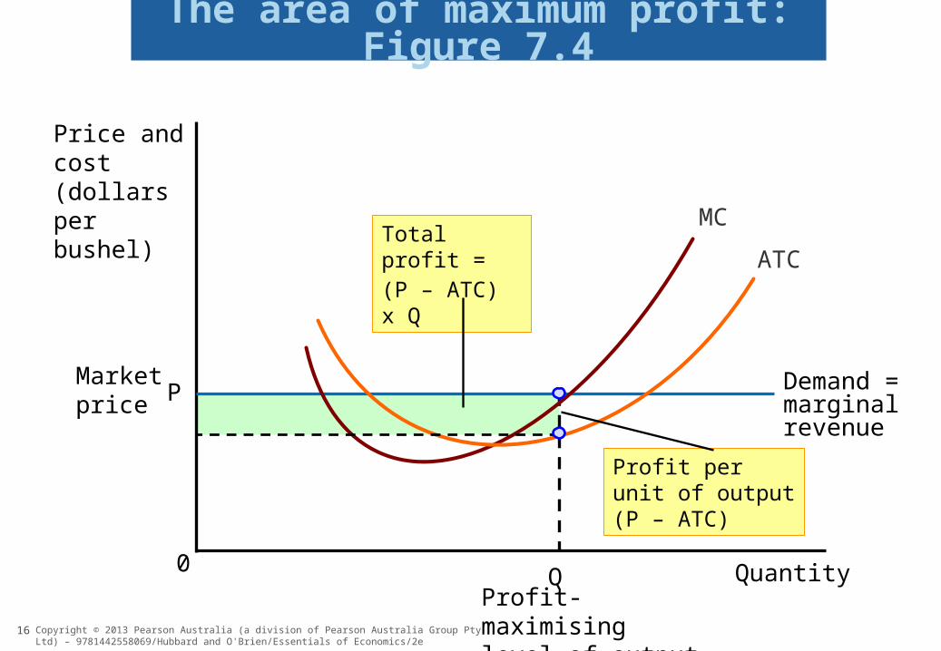
Illustrating profit or loss on the cost curve graph
Profit = (P x Q) TC
or
Profit per unit =
Total profit = (P ATC) x Q
Q
Q)(P
QProfit
QTC
ATCPQ
Profit
Copyright © 2013 Pearson Australia (a division of Pearson Australia Group Pty Ltd) – 9781442558069/Hubbard and O'Brien/Essentials of Economics/2e 15
Price and cost (dollars per bushel)
Quantity0
Demand = marginal revenue
P
Q
Market price
Profit-maximising level of output
MC
ATCTotal profit = (P – ATC) x Q
Profit per unit of output (P – ATC)
Copyright © 2013 Pearson Australia (a division of Pearson Australia Group Pty Ltd) – 9781442558069/Hubbard and O'Brien/Essentials of Economics/2e
16
The area of maximum profit: Figure 7.4

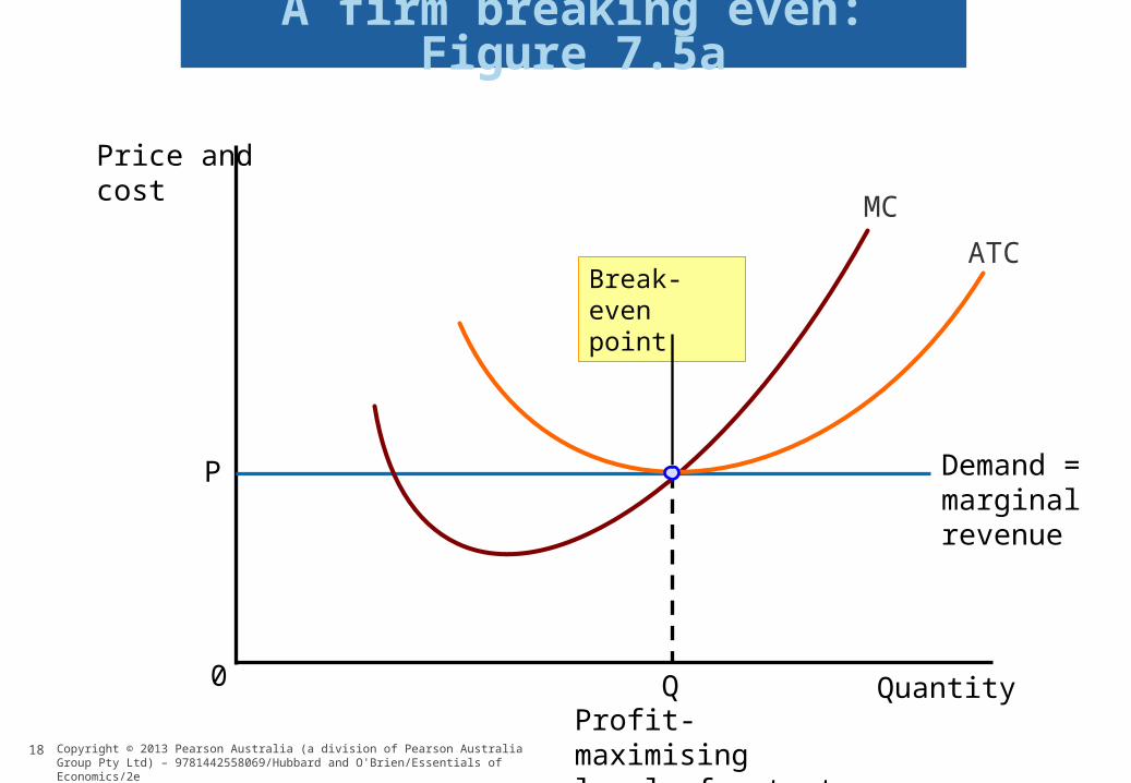
Illustrating when a firm is breaking even or operating at a loss
If P > ATC; the firm makes a profit.
If P = ATC; the firm breaks even (its per unit cost equals per unit revenue; thus, the firm’s total cost equals its total revenue).
If P < ATC; the firm experiences losses.Copyright © 2013 Pearson Australia (a division of Pearson Australia Group Pty Ltd) – 9781442558069/Hubbard and O'Brien/Essentials of Economics/2e 17
Illustrating profit or loss on the cost curve graph
Quantity0
Demand = marginal revenue
P
QProfit-maximising level of output
MC
ATCBreak-even point
Price and cost
Copyright © 2013 Pearson Australia (a division of Pearson Australia Group Pty Ltd) – 9781442558069/Hubbard and O'Brien/Essentials of Economics/2e
18
A firm breaking even: Figure 7.5a

Price and cost
0
Demand = marginal revenue
P
QLoss minimising level of output
MC
ATC
Losses
ATC
Quantity
Copyright © 2013 Pearson Australia (a division of Pearson Australia Group Pty Ltd) – 9781442558069/Hubbard and O'Brien/Essentials of Economics/2e
19
A firm experiencing losses: Figure 7.5b
In the short run, a firm suffering losses has two choices:
– Continue to produce
– Stop production by shutting down temporarily
Sunk cost: A cost that has already been paid and cannot be recovered.
Deciding whether to produce or to shut down in the short run
Copyright © 2013 Pearson Australia (a division of Pearson Australia Group Pty Ltd) – 9781442558069/Hubbard and O'Brien/Essentials of Economics/2e 20

The supply curve of a firm in the short run
For any given price, the marginal cost curve shows the quantity of output that a firm will supply.
Therefore, the perfectly competitive firm’s marginal cost curve is also its supply curve—but only for prices at or above average variable cost.
Copyright © 2013 Pearson Australia (a division of Pearson Australia Group Pty Ltd) – 9781442558069/Hubbard and O'Brien/Essentials of Economics/2e
Deciding whether to produce or to shut down in the short run
21

The supply curve of a firm in the short run, cont.
Even if a firm suffers losses, it should continue to operate as long as P > AVC.
Shutdown point: The minimum point on a firm’s average variable cost curve; if the price falls below this point, the firm shuts down production in the short run.
– Shutdown point: P < AVC
Copyright © 2013 Pearson Australia (a division of Pearson Australia Group Pty Ltd) – 9781442558069/Hubbard and O'Brien/Essentials of Economics/2e
Deciding whether to produce or to shut down in the short run
22

Price and cost
Quantity0
PMIN
QSD
MCATC
Shutdown point
AVCThe minimum price at which the firm will continue to produce
The supply curve for the firm in the short run
Copyright © 2013 Pearson Australia (a division of Pearson Australia Group Pty Ltd) – 9781442558069/Hubbard and O'Brien/Essentials of Economics/2e
The firm’s short-run supply curve: Figure 7.6
23

The market supply curve in a perfectly competitive industry
The market supply curve is derived from individual firms’ marginal cost curves.
Copyright © 2013 Pearson Australia (a division of Pearson Australia Group Pty Ltd) – 9781442558069/Hubbard and O'Brien/Essentials of Economics/2e
Deciding whether to produce or to shut down in the short run
24
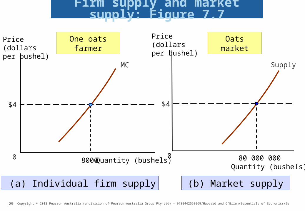
(b) Market supply
0
(a) Individual firm supply
Quantity (bushels)
MC
$4
8000
Price (dollars per bushel)
Price (dollars per bushel)
Quantity (bushels)
0
$4
Oats marketOne oats farmer
80 000 000
Supply
25 Copyright © 2013 Pearson Australia (a division of Pearson Australia Group Pty Ltd) – 9781442558069/Hubbard and O'Brien/Essentials of Economics/2e
Firm supply and market supply: Figure 7.7

The entry and exit of firms in the long run
Economic profit and the entry or exit decision
Economic profit: A firm’s revenues minus all its costs, implicit and explicit.
Economic profit in a perfectly competitive industry is only a short-run occurrence.
Economic profit leads to the entry of new firms into the industry.
26 Copyright © 2013 Pearson Australia (a division of Pearson Australia Group Pty Ltd) – 9781442558069/Hubbard and O'Brien/Essentials of Economics/2e

Explicit costs
Water $10 000
Wages $15 000
Organic fertiliser $10 000
Electricity $ 5 000
Payment on bank loan $45 000
Implicit costs
Foregone salary $30 000
Opportunity cost of the $100 000 she has invested in her farm
$10 000
Total cost $125 000
27 Copyright © 2013 Pearson Australia (a division of Pearson Australia Group Pty Ltd) – 9781442558069/Hubbard and O'Brien/Essentials of Economics/2e
Costs per year for Anne Moreno’s organic food farm: Table 7.4

28 Copyright © 2013 Pearson Australia (a division of Pearson Australia Group Pty Ltd) – 9781442558069/Hubbard and O'Brien/Essentials of Economics/2e
The effect of entry on economic profits: Figure 7.8

Economic profit and the entry or exit decision, cont.
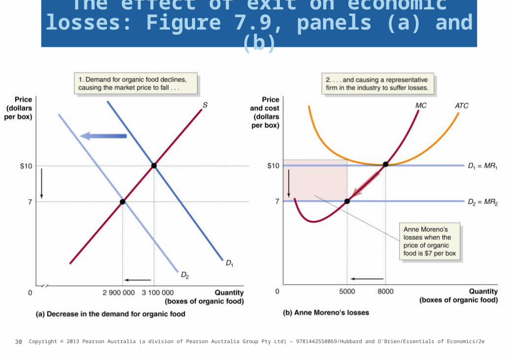
Economic loss: The situation in which a firm’s total revenue is less than its total cost, including all implicit costs.
Economic loss in a perfectly competitive industry is only a short-run occurrence.
Economic loss leads to the exit of some firms from the industry.
29 Copyright © 2013 Pearson Australia (a division of Pearson Australia Group Pty Ltd) – 9781442558069/Hubbard and O'Brien/Essentials of Economics/2e
LEARNING OBJECTIVE 5
The entry and exit of firms in the long run
Copyright © 2013 Pearson Australia (a division of Pearson Australia Group Pty Ltd) – 9781442558069/Hubbard and O'Brien/Essentials of Economics/2e
The effect of exit on economic losses: Figure 7.9, panels (a) and (b)
30

Copyright © 2013 Pearson Australia (a division of Pearson Australia Group Pty Ltd) – 9781442558069/Hubbard and O'Brien/Essentials of Economics/2e
The effect of exit on economic losses: Figure 7.9, panels (c) and (d)
31

Long-run equilibrium in a perfectly competitive market
Long-run competitive equilibrium: The situation in which the entry and exit of firms has resulted in the typical firm breaking even.
The long-run equilibrium market price is at the minimum point on the typical firm’s average total cost curve.
32 Copyright © 2013 Pearson Australia (a division of Pearson Australia Group Pty Ltd) – 9781442558069/Hubbard and O'Brien/Essentials of Economics/2e
LEARNING OBJECTIVE 5
The entry and exit of firms in the long run

Long-run equilibrium in a perfectly competitive market, cont.
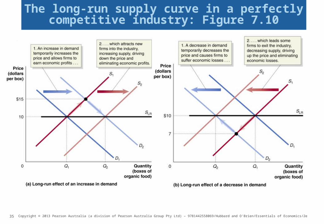
Long-run supply curve: A curve showing the relationship in the long run between market price and the quantity supplied.
The long-run supply curve will be horizontal at the market price.
33 Copyright © 2013 Pearson Australia (a division of Pearson Australia Group Pty Ltd) – 9781442558069/Hubbard and O'Brien/Essentials of Economics/2e
The entry and exit of firms in the long run

Long-run equilibrium in a perfectly competitive market, cont.
In the long run, a perfectly competitive market will supply whatever amount of a good consumers demand at a price determined by the minimum point on the typical firm’s average total cost curve.
34 Copyright © 2013 Pearson Australia (a division of Pearson Australia Group Pty Ltd) – 9781442558069/Hubbard and O'Brien/Essentials of Economics/2e
The entry and exit of firms in the long run
35 Copyright © 2013 Pearson Australia (a division of Pearson Australia Group Pty Ltd) – 9781442558069/Hubbard and O'Brien/Essentials of Economics/2e
The long-run supply curve in a perfectly competitive industry: Figure 7.10
Increasing-cost and decreasing-cost industries
Constant-cost industry: An industry in which a firm’s average costs do not change as the industry expands (horizontal long-run supply curve).
Increasing-cost industry: An industry in which a firm’s average costs rise as the industry expands (upward-sloping long-run supply curve).
Decreasing-cost industry: An industry in which a firm’s average costs fall as the industry expands (downward-sloping long-run supply curve).
36 Copyright © 2013 Pearson Australia (a division of Pearson Australia Group Pty Ltd) – 9781442558069/Hubbard and O'Brien/Essentials of Economics/2e
The entry and exit of firms in the long run

Perfect competition and efficiency Productive efficiency: When a good or service is
produced using the least amount of resources.
Allocative efficiency:Firms will supply all those goods that provide consumers with a marginal benefit at least as great as the marginal cost of producing them:
– The price of a good represents the marginal benefit consumers receive from the last unit of the good consumed.
– Perfectly competitive firms produce up to the point where the price of the good equals the marginal cost of producing the last unit.
– Therefore, firms produce up to the point where the last unit provides a marginal benefit to consumers equal to the marginal cost of producing it.
37 Copyright © 2013 Pearson Australia (a division of Pearson Australia Group Pty Ltd) – 9781442558069/Hubbard and O'Brien/Essentials of Economics/2e

Allocative efficiency
Firms will supply all those goods that provide consumers with a marginal benefit at least as great as the marginal cost of producing them:
– The price of a good represents the marginal benefit consumers receive from the last unit of the good consumed.
– Perfectly competitive firms produce up to the point where the price of the good equals the marginal cost of producing the last unit.
– Therefore, firms produce up to the point where the last unit provides a marginal benefit to consumers equal to the marginal cost of producing it.
38 Copyright © 2013 Pearson Australia (a division of Pearson Australia Group Pty Ltd) – 9781442558069/Hubbard and O'Brien/Essentials of Economics/2e
Perfect competition and efficiency

Dynamic efficiency: Occurs when new technologies and innovation are adopted over time, and when firms adapt their product to changes in consumer preferences and tastes.
– When striving for dynamic efficiency, firms will use new technology and thereby reduce production costs (productive efficiency).
– By adapting their product to changes in consumer preferences, firms will produce goods and services consumers value the most (allocative efficiency).
39 Copyright © 2013 Pearson Australia (a division of Pearson Australia Group Pty Ltd) – 9781442558069/Hubbard and O'Brien/Essentials of Economics/2e
Perfect competition and efficiency


