Lecture 4: Complex Numbers Functions, and Data Input Scripts and Functions_big.pdf ·...

Lecture 4: Complex Numbers Functions, and Data Input

Dr. Mohammed HawaElectrical Engineering Department

University of Jordan

EE201: Computer Applications. See Textbook Chapter 3.

Copyright © Dr. Mohammed Hawa Electrical Engineering Department, University of Jordan

What is a Function?

• A MATLAB Function (e.g. y = func(x1, x2)) is like a script file, but with inputs and outputs provided automatically in the commend window.

• In MATLAB, functions can take zero, one, two or more inputs, and can provide zero, one, two or more outputs.

• There are built-in functions (written by the MATLAB team) and functions that you can define (written by you and stored in .m file).

• Functions can be called from command line, from wihtin a script, or from another function.

2

Copyright © Dr. Mohammed Hawa Electrical Engineering Department, University of Jordan 3


Functions are Helpful

• Enable “divide and conquer” strategy– Programming task broken into smaller tasks

• Code reuse– Same function useful for many problems

• Easier to debug– Check right outputs returned for all possible

inputs

• Hide implementation– Only interaction via inputs/outputs, how it is

done (implementation) hidden inside the function.

4


Finding Useful Functions

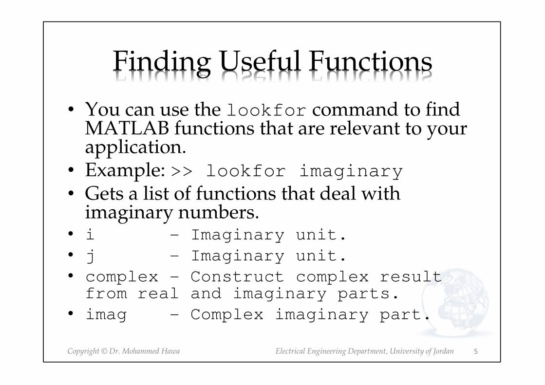
• You can use the lookfor command to find MATLAB functions that are relevant to your application.

• Example: >> lookfor imaginary

• Gets a list of functions that deal with imaginary numbers.

• i - Imaginary unit.

• j - Imaginary unit.

• complex - Construct complex result from real and imaginary parts.

• imag - Complex imaginary part.

5


Calling Functions

• Function names are case sensitive (meshgrid, meshGrid and MESHGRID are interpreted as different functions).

• Inputs (called function arguments or function parameters) can be either numbers or variables.

• Inputs are passed into the function inside of parentheses () separated by commas.

• We usually assign the output to variable(s) so we can use it later. Otherwise it is assigned to the built-in variable ans.

6


Rules

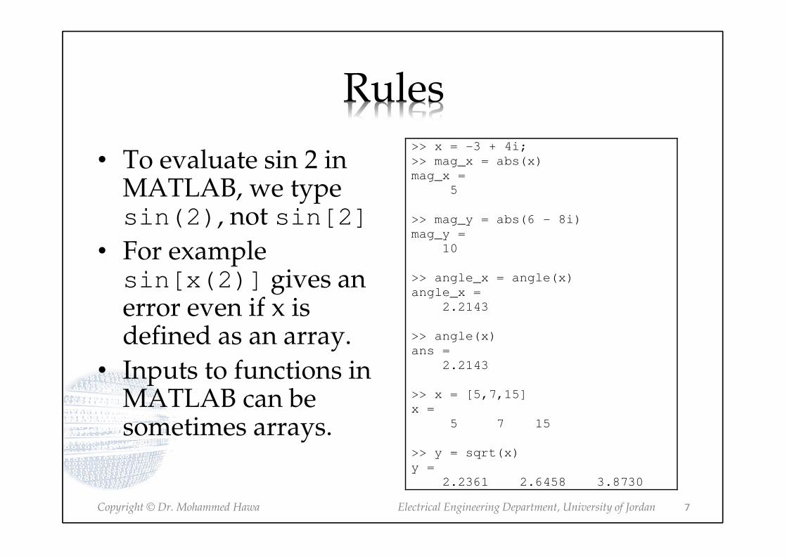
• To evaluate sin 2 in MATLAB, we type sin(2), not sin[2]

• For example sin[x(2)] gives an error even if x is defined as an array.

• Inputs to functions in MATLAB can be sometimes arrays.

>> x = -3 + 4i;

>> mag_x = abs(x)

mag_x =

5

>> mag_y = abs(6 - 8i)

mag_y =

10

>> angle_x = angle(x)

angle_x =

2.2143

>> angle(x)

ans =

2.2143

>> x = [5,7,15]

x =

5 7 15

>> y = sqrt(x)

y =

2.2361 2.6458 3.8730

7


Function Composition

• Composition: Using a function as an argument of another function

• Allowed in MATLAB.

• Just check the number and placement of parentheses when typing such expressions.

• sin(sqrt(x)+1)

• log(x.^2 + sin(5))

8


Which expression is correct?

• You want to find sin� � . What do you write?

• (sin(x))^2

• sin^2(x)

• sin^2x

• sin(x^2)

• sin(x)^2

• Solution: Only first and last expressions are correct.

9


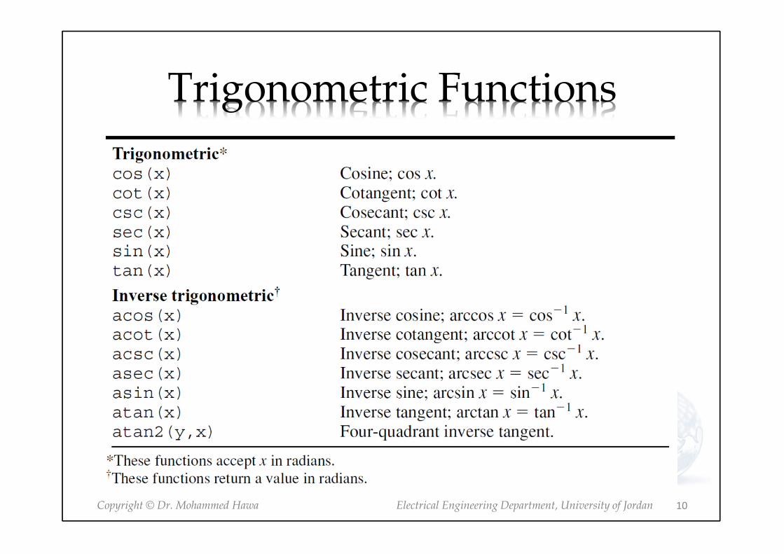
Trigonometric Functions

10


Hyperbolic functions

11


User-Defined Functions

• Functions must be saved to a file with .m extension. • Filename (without the .m) must match EXACTLY

the function name.• First line in the file must begin with a function

definition line that illustrates inputs and outputs.

function [output variables] = name(input variables)

• This line distinguishes a function M-file from a script M-file.

• Output variables are enclosed in square brackets.• Input variables must be enclosed with parentheses.

12


Functions Names

• Function names may only use alphanumeric characters and the underscore.

• Functions names should NOT:– include spaces

– start with a number

– use the same name as an existing command

• Consider adding a header comment, just under the function definition (for help).

13


Exercise: Your Own pol2cart

• Make sure you set you Current Folder to Desktop (or where you saved the .m file).

14


Test your newly defined function

>> [a, b] = polar_to_cartesian(3, pi)

a =

-3

b =

3.6739e-016

>> polar_to_cartesian(3, pi)

ans =

-3

>> [a, b] = polar_to_cartesian(3, pi/4)

a =

2.1213

b =

2.1213

>> [a, b] = polar_to_cartesian([3 3 3], [pi pi/4 pi/2])

a =

-3.0000 2.1213 0.0000

b =

0.0000 2.1213 3.0000

15


MATLAB has pol2cart>> help pol2cart

POL2CART Transform polar to Cartesian coordinates.

[X,Y] = POL2CART(TH,R) transforms corresponding elements of data

stored in polar coordinates (angle TH, radius R) to Cartesian

coordinates X,Y. The arrays TH and R must the same size (or

either can be scalar). TH must be in radians.

[X,Y,Z] = POL2CART(TH,R,Z) transforms corresponding elements of

data stored in cylindrical coordinates (angle TH, radius R, height

Z) to Cartesian coordinates X,Y,Z. The arrays TH, R, and Z must be

the same size (or any of them can be scalar). TH must be in radians.

Class support for inputs TH,R,Z:

float: double, single

See also cart2sph, cart2pol, sph2cart.

Reference page in Help browser

doc pol2cart

16


Just like your code!>> type pol2cart

function [x,y,z] = pol2cart(th,r,z)

%POL2CART Transform polar to Cartesian coordinates.

% [X,Y] = POL2CART(TH,R) transforms corresponding elements of data

% stored in polar coordinates (angle TH, radius R) to Cartesian

% coordinates X,Y. The arrays TH and R must the same size (or

% either can be scalar). TH must be in radians.

%

% [X,Y,Z] = POL2CART(TH,R,Z) transforms corresponding elements of

% data stored in cylindrical coordinates (angle TH, radius R, height

% Z) to Cartesian coordinates X,Y,Z. The arrays TH, R, and Z must be

% the same size (or any of them can be scalar). TH must be in radians.

%

% Class support for inputs TH,R,Z:

% float: double, single

%

% See also CART2SPH, CART2POL, SPH2CART.

% L. Shure, 4-20-92.

% Copyright 1984-2004 The MathWorks, Inc.

% $Revision: 5.9.4.2 $ $Date: 2004/07/05 17:02:08 $

x = r.*cos(th);

y = r.*sin(th);

17


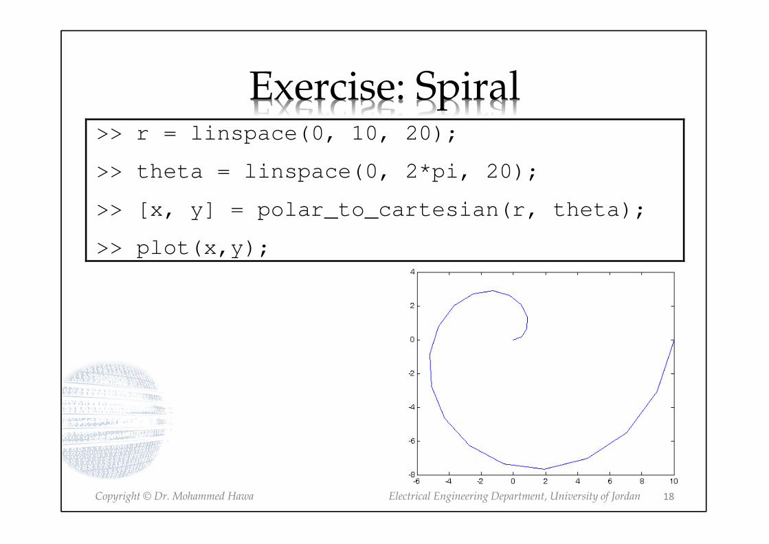
Exercise: Spiral>> r = linspace(0, 10, 20);

>> theta = linspace(0, 2*pi, 20);

>> [x, y] = polar_to_cartesian(r, theta);

>> plot(x,y);

18


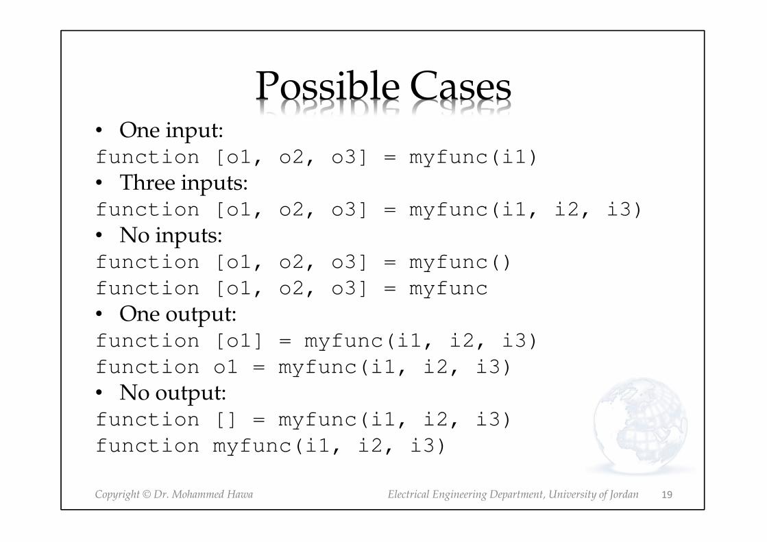
Possible Cases• One input:function [o1, o2, o3] = myfunc(i1)

• Three inputs:function [o1, o2, o3] = myfunc(i1, i2, i3)

• No inputs:function [o1, o2, o3] = myfunc()

function [o1, o2, o3] = myfunc

• One output:function [o1] = myfunc(i1, i2, i3)

function o1 = myfunc(i1, i2, i3)

• No output:function [] = myfunc(i1, i2, i3)

function myfunc(i1, i2, i3)

19


Local Variables

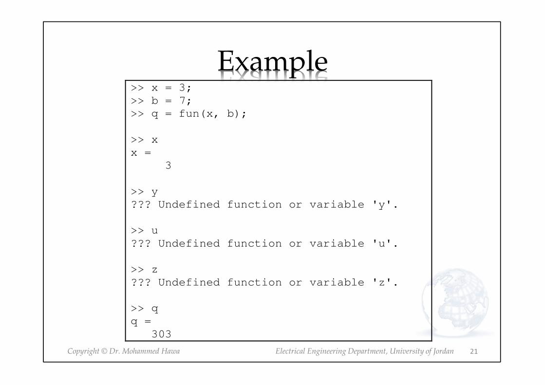
• The variables x, y, u, z are local to the function fun, so their values will not be available in the workspace outside the function.

• See example below.

function z = fun(x,y)

u = 3*x;

z = u + 6*y.^2;

% return missing is fine at end of file

20


Example>> x = 3;

>> b = 7;

>> q = fun(x, b);

>> x

x =

3

>> y

??? Undefined function or variable 'y'.

>> u

??? Undefined function or variable 'u'.

>> z

??? Undefined function or variable 'z'.

>> q

q =

303

21


Exercise

function show_date

clear

clc

date

% how many inputs and outputs do we have?

22


Homework

function [dist, vel] = drop(vO, t) % Compute the distance travelled and the % velocity of a dropped object, from % the initial velocity vO, and time t % Author: Dr. Mohammed Hawa

g = 9.80665; % gravitational acceleration (m/s^2) vel = g*t + vO; dist = 0.5*g*t.^2 + vO*t;

>> t = 0:0.1:5;

>> [distance_dropped, velocity] = drop(10, t);

>> plot(t, velocity)

23


Local vs. Global Variables

• The variables inside a function are local. Their scope is only inside the function that declares them.

• In other words, functions create their own workspaces.• Function inputs are also created in this workspace

when the function starts.• Functions do not know about any variables in any

other workspace.• Function outputs are copied from the function

workspace when the function ends.• Function workspaces are destroyed after the function

ends.– Any variables created inside the function “disappear”

when the function ends.

24


Local vs. Global Variables

• You can, however, define global variables if you want using the global keyword.

• Syntax: global a x q

• Global variables are available to the basic workspace and to other functions that declare those variables global (allowing assignment to those variables from multiple functions).

25


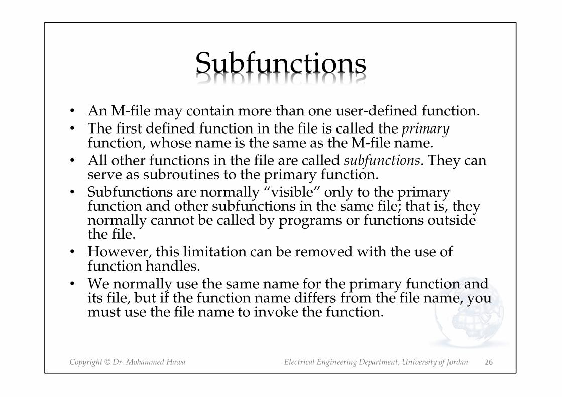
Subfunctions

• An M-file may contain more than one user-defined function.• The first defined function in the file is called the primary

function, whose name is the same as the M-file name. • All other functions in the file are called subfunctions. They can

serve as subroutines to the primary function.• Subfunctions are normally “visible” only to the primary

function and other subfunctions in the same file; that is, they normally cannot be called by programs or functions outside the file.

• However, this limitation can be removed with the use of function handles.

• We normally use the same name for the primary function and its file, but if the function name differs from the file name, you must use the file name to invoke the function.

26


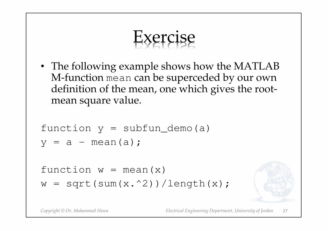
Exercise

• The following example shows how the MATLAB M-function mean can be superceded by our own definition of the mean, one which gives the root-mean square value.

function y = subfun_demo(a)

y = a - mean(a);

function w = mean(x)

w = sqrt(sum(x.^2))/length(x);

27


Example

• A sample session follows.

>>y = subfn_demo([4 -4])

y =

1.1716 -6.8284

• If we had used the MATLAB M-function mean, we would have obtained a different answer; that is,

>>a = [4 -4];

>>b = a - mean(a)

b =

4 -4

28


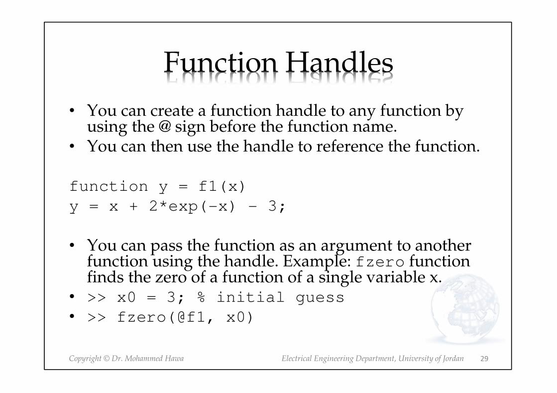
Function Handles

• You can create a function handle to any function by using the @ sign before the function name.

• You can then use the handle to reference the function.

function y = f1(x)

y = x + 2*exp(-x) - 3;

• You can pass the function as an argument to another function using the handle. Example: fzero function finds the zero of a function of a single variable x.

• >> x0 = 3; % initial guess

• >> fzero(@f1, x0)

29


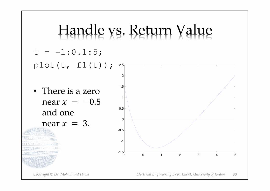
Handle vs. Return Value

t = -1:0.1:5;

plot(t, f1(t));

• There is a zero near � � �0.5

and one near � � 3.

-1 0 1 2 3 4 5-1.5

-1

-0.5

0

0.5

1

1.5

2

2.5

30


Exercise

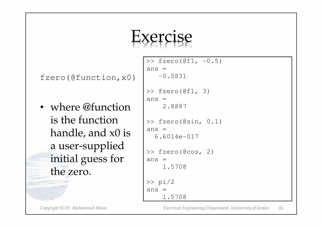
fzero(@function,x0)

• where @function is the function handle, and x0 is a user-supplied initial guess for the zero.

>> fzero(@f1, -0.5)

ans =

-0.5831

>> fzero(@f1, 3)

ans =

2.8887

>> fzero(@sin, 0.1)

ans =

6.6014e-017

>> fzero(@cos, 2)

ans =

1.5708

>> pi/2

ans =

1.5708

31


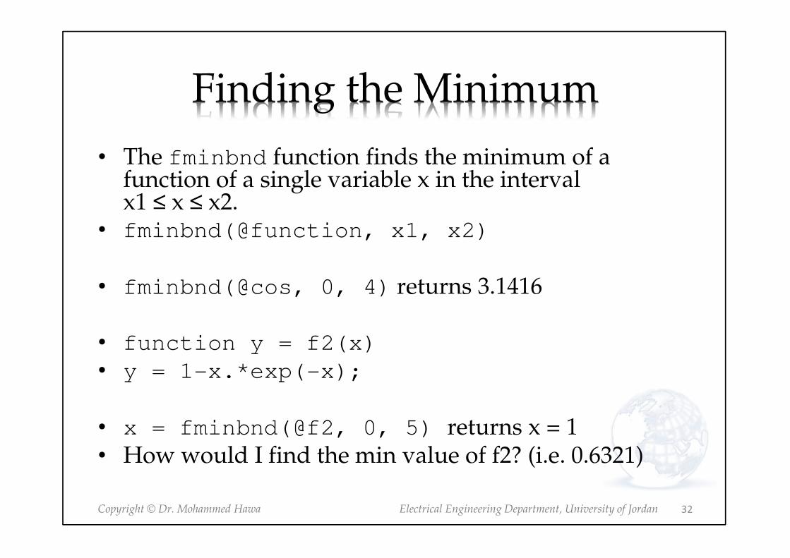
Finding the Minimum

• The fminbnd function finds the minimum of a function of a single variable x in the interval x1 ≤ x ≤ x2.

• fminbnd(@function, x1, x2)

• fminbnd(@cos, 0, 4) returns 3.1416

• function y = f2(x)

• y = 1-x.*exp(-x);

• x = fminbnd(@f2, 0, 5) returns x = 1 • How would I find the min value of f2? (i.e. 0.6321)

32


Exercise

• For the function:

• � 0.025�� 0.0625�� 0.333��

• Find the minimum inthe intervals:

• � ∈ �1, 4

• � ∈ 1, 4

• � ∈ 2, 4

• � ∈ �1, 1

33


Old vs. New

• New syntax for function handles:

fzero(@f1, -0.5)

• Older syntax for function handles :

fzero('f1', -0.5)

• The new syntax is preferred, though both will work just fine.

• Which one gives the correct answer:fzero('sin', 3)or fzero(@sin, 3)

34


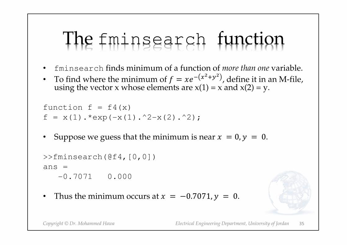
The fminsearch function

• fminsearch finds minimum of a function of more than one variable.

• To find where the minimum of � � �� , define it in an M-file, using the vector x whose elements are x(1) = x and x(2) = y.

function f = f4(x)

f = x(1).*exp(-x(1).^2-x(2).^2);

• Suppose we guess that the minimum is near � � 0, � � 0.

>>fminsearch(@f4,[0,0])

ans =

-0.7071 0.000

• Thus the minimum occurs at � � 0.7071, � � 0.

35


Inline Function

• No need to save the function in an M-file.

• Useful for small size functions defined on the fly.

• You can use a string array to define the function.

• Anonymous functions are similar (see next).

>> f4 = inline('x.^2-4')

f4 =

Inline function:

f4(x) = x.^2-4

>> [x, value] = fzero(f4, 0)

x =

-2

value =

0

>> f5str = 'x.^2-4'; % string array

>> f5 = inline(f5str)

f5 =

Inline function:

f5(x) = x.^2-4

>> x = fzero(f5, 3)

x =

2

>> x = fzero('x.^2-4', 3)

x =

2

>> f6 = inline('x.*y')

f6 =

Inline function:

f6(x,y) = x.*y

36


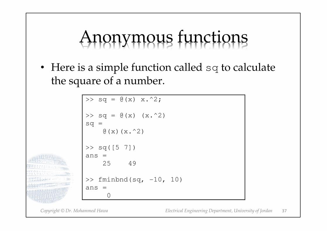
Anonymous functions

• Here is a simple function called sq to calculate the square of a number.

>> sq = @(x) x.^2;

>> sq = @(x) (x.^2)

sq =

@(x)(x.^2)

>> sq([5 7])

ans =

25 49

>> fminbnd(sq, -10, 10)

ans =

0

37


Exercise>> sqrtsum = @(x,y) sqrt(x.^2 + y.^2);

>> sqrtsum(3, 4)

ans =

5

>> A = 6; B = 4;

>> plane = @(x,y) A*x + B*y;

>> z = plane(2,8)

z =

44

>> f = @(x) x.^3; % try by hand!

>> g = @(x) 5*sin(x);

>> h = @(x) g(f(x));

>> h(2)

ans =

4.9468

38


Variables in Anonymous Functions

• When the function is created MATLAB, it captures the values of these variables and retains those values for the lifetime of the function handle. If the values of A or B are changed after the handle is created, their values associated with the handle do not change.

• This feature has both advantages and disadvantages, so you must keep it in mind.

39


For Speed Use Handles

• The function handle provides speed improvements.

• Another advantage of using a function handle is that it provides access to subfunctions, which are normally not visible outside of their defining M-file.

40


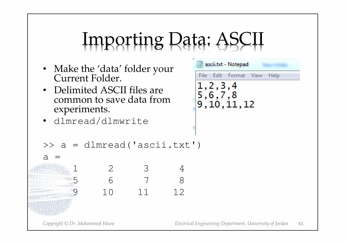
Importing Data: ASCII

• Make the ‘data’ folder your Current Folder.

• Delimited ASCII files are common to save data fromexperiments.

• dlmread/dlmwrite

>> a = dlmread('ascii.txt')

a =

1 2 3 4

5 6 7 8

9 10 11 12

41


Importing Data: Excel


• MATLAB can also read and write to Excel Files.

• xlsread/xlswrite

>> a = xlsread('data.xls')

a =

10 30 50 60

15 20 25 30

30 31 32 33

80 82 84 86

42


Importing Data: Images


• Read and write images:

• imread/imwrite

>> c = imread('cat.jpg');

>> imshow(c);

>>

>> imshow(255-c); % inverse

43


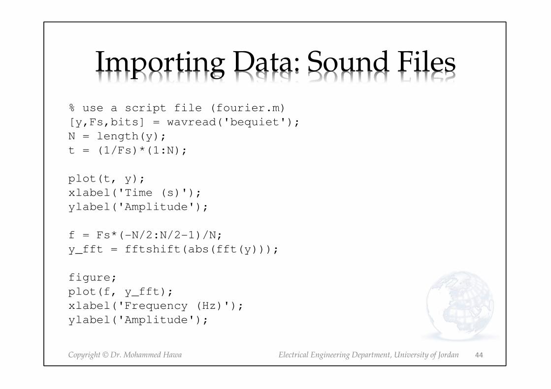
Importing Data: Sound Files

% use a script file (fourier.m)

[y,Fs,bits] = wavread('bequiet');

N = length(y);

t = (1/Fs)*(1:N);

plot(t, y);

xlabel('Time (s)');

ylabel('Amplitude');

f = Fs*(-N/2:N/2-1)/N;

y_fft = fftshift(abs(fft(y)));

figure;

plot(f, y_fft);

xlabel('Frequency (Hz)');

ylabel('Amplitude');

44


bequiet.wav (BW of human voice!)

0 0.2 0.4 0.6 0.8 1 1.2 1.4-1

-0.8

-0.6

-0.4

-0.2

0

0.2

0.4

0.6

0.8

1

Time (s)

Am

plit

ude

-6000 -4000 -2000 0 2000 4000 60000

50

100

150

Frequency (Hz)A

mplit

ude

45


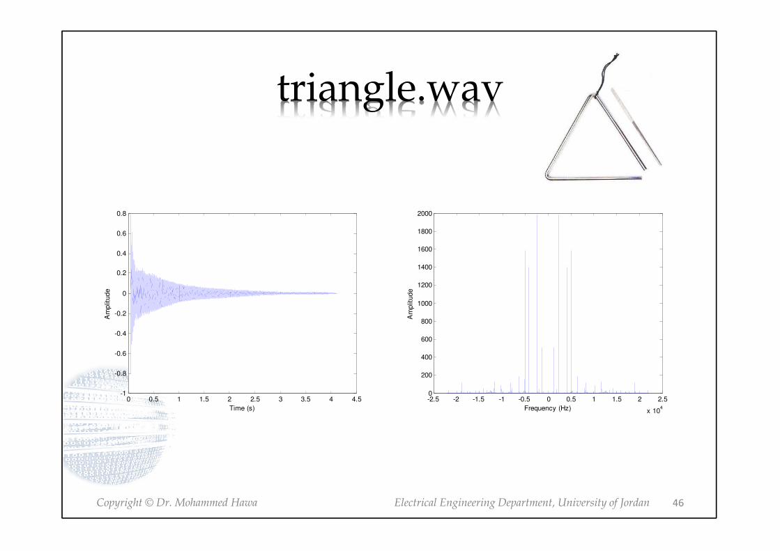
triangle.wav

0 0.5 1 1.5 2 2.5 3 3.5 4 4.5-1

-0.8

-0.6

-0.4

-0.2

0

0.2

0.4

0.6

0.8

Time (s)

Am

plit

ude

-2.5 -2 -1.5 -1 -0.5 0 0.5 1 1.5 2 2.5

x 104

0

200

400

600

800

1000

1200

1400

1600

1800

2000

Frequency (Hz)A

mplit

ude

46


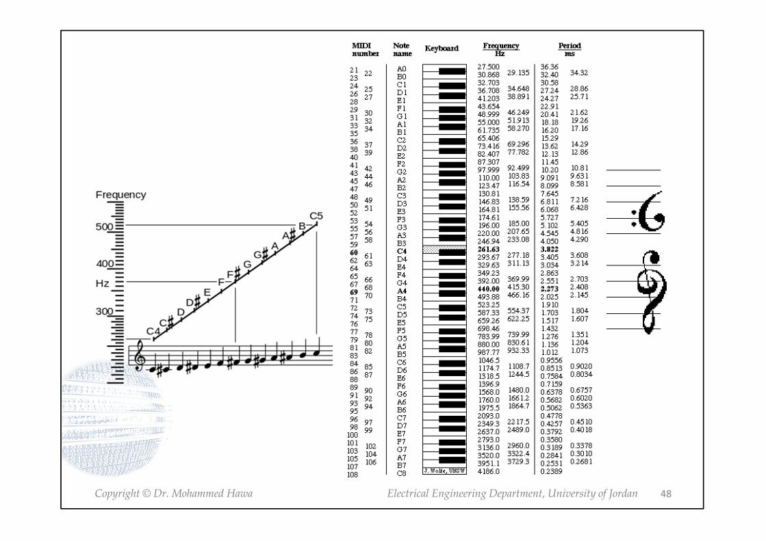
tuningA4.wav (frequency?)

0 1 2 3 4 5 6 7 8 9-0.4

-0.3

-0.2

-0.1

0

0.1

0.2

0.3

Time (s)

Am

plit

ude

-1.5 -1 -0.5 0 0.5 1 1.5

x 104

0

500

1000

1500

2000

2500

3000

3500

4000

4500

Frequency (Hz)A

mplit

ude

47

Copyright © Dr. Mohammed Hawa Electrical Engineering Department, University of Jordan 48


guitar.wav

0 0.5 1 1.5 2 2.5-1

-0.8

-0.6

-0.4

-0.2

0

0.2

0.4

0.6

0.8

Time (s)

Am

plit

ude

-2.5 -2 -1.5 -1 -0.5 0 0.5 1 1.5 2 2.5

x 104

0

200

400

600

800

1000

1200

1400

1600

1800

Frequency (Hz)A

mplit

ude

49


Homework

• Solve as many problems from Chapter 3 as you can

• Suggested problems:

• 3.1, 3.3, 3.6, 3.9, 3.14, 3.18, 3.24

50

Date post:	16-Jan-2020
Category:	Documents
Upload:	others
View:	17 times
Download:	0 times

Lecture 4: Complex Numbers Functions, and Data Input Scripts and Functions_big.pdf ·...

Documents