42
University of Illinois at Urbana-Champaign Lecture 4: Dynamical and Hybrid Systems Sayan Mitra
University of Illinoisat Urbana-Champaign
Lecture4:DynamicalandHybridSystems
SayanMitra

IntroductiontodynamicalsystemsBehaviorsofphysicalprocessesaredescribedintermsofinstantaneouslaws
Commonnotation: ÇÈ »Ç»
= 𝑓 𝑥 𝑡 , 𝑢 𝑡 , 𝑡 − 1 ,wheretime𝑡 ∈ ℝ;state𝑥 𝑡 ∈ ℝ�; 𝑖𝑛𝑝𝑢𝑡𝑢 𝑡 ∈ℝÊ; 𝑓: ℝ�×ℝÊ×ℝ → ℝ�
Initialvalueproblem:Givensystem(1)andinitialstate𝑥[ ∈ ℝ�, 𝑡[ ∈ ℝ,andinputu:ℝ → ℝÊ, findastatetrajectoryorsolutionof(1).

NotionsofsolutionWhatisasolution?Manydifferentnotions.
Definition1.(Firstattempt)Given 𝑥[ and 𝑢, 𝜉: ℝ → ℝ�isasolutionortrajectoryiff (1)𝜉 𝑡[ = 𝑥[ and(2)ÇÇ»𝜉 𝑡 = 𝑓(𝜉 𝑡 , 𝑢 𝑡 , 𝑡)), ∀𝑡 ∈ ℝ.
Mathematicallymakessense,buttoorestrictive.Assumesthat𝜉 isnotonlycontinuous,butalsodifferentiable.Thisdisallowsu(𝑡) tobediscontinuous,whichisoftenrequiredforoptimalcontrol.

ModifiednotionDefinition.𝑢 ⋅ isapiece-wisecontinuouswithsetofdiscontinuitypoints𝐷 ⊆ ℝÊ if(1) ∀𝜏 ∈ 𝐷, lim
»→Ñ�𝑢 𝑡 < ∞; lim
»→ÑÓ𝑢 𝑡 < ∞
(2) Continuousfromright lim»→Ñ�
𝑢 𝑡 = 𝑢 𝑡(3) ∀𝑡[ < 𝑡M , 𝑡[, 𝑡M ∩ 𝐷 isfinite
𝑃𝐶( 𝑡[, 𝑡M , ℝÊ)isthesetofallpiece-wisecontinuousfunctionsoverthedomain 𝑡[, 𝑡M
Define𝑝 𝜉 𝑡 , 𝑡 = 𝑓 𝑥 𝑡 , 𝑢 𝑡 , 𝑡 , foragiven𝑢 𝑡 . Since𝑢 𝑡 isPCin𝑡 sois𝑝 inthesecondargument.
Definition2.Given𝑥[ and𝑢, 𝜉: ℝ → ℝ� isasolutionortrajectoryiff (1)𝜉 𝑡[ = 𝑥[ and(2)ÇÇ»𝜉 𝑡 = 𝑝(𝜉 𝑡 , 𝑡), ∀𝑡 ∈ ℝ\D.
𝜏M 𝜏P
𝑢 𝑡

IsPCinput𝑢 𝑡 adequateforguaranteeingexistenceofsolutions?
Example.�� 𝑡 = −𝑠𝑔𝑛 𝑥 𝑡 ; 𝑥[ = 𝑐; 𝑡[ = 0; 𝑐 > 0Solution:𝜉 𝑡 = 𝑐 − 𝑡 for𝑡 ≤ 𝑐;check𝜉 = −1Problem:𝑓 discontinuousis𝑥
Example.�� 𝑡 = 𝑥P; 𝑥[ = 𝑐; 𝑡[ = 0; 𝑐 > 0Solution:𝜉 𝑡 = �
M#»�worksfor𝑡 < 1/𝑐;check𝜉
Problem:As𝑡 → M�then𝑥 𝑡 → ∞;𝑝 growstoofast

Lipschitzcontinuity
Afunction𝑓:ℝ� → ℝ isLipschitzcontinuousifthereexist𝐿 > 0 suchthatforanypair𝑥, 𝑥′ ∈ℝ�, 𝑓 𝑥 − 𝑓 𝑥′ ≤ 𝐿 𝑥 − 𝑥t
Examples:6𝑥 + 4; 𝑥 ; alldifferentiablefunctionswithboundedderivatives
Non-examples: 𝑥� ; 𝑥P (locallyLipschitz)

Existenceanduniquenessofsolutions
Theorem.If𝑝(𝑥 𝑡 , 𝑥) isLipschitzcontinuousinthefirstargumentthen(1)hasuniquesolutions.
Transitionsystemmodel

Lineartime-varyingsystemsIngeneral,fornonlineardynamicalsystemswedonothaveclosedformsolutionsfor𝜉 𝑡 , buttherearenumericalsolverslikeCAPD,VNODE
�� 𝑡 = 𝐴 𝑡 𝑥 𝑡 + 𝐵 𝑡 𝑢 𝑡 --- (2)𝑦 𝑡 = 𝐶 𝑡 𝑥 𝑡 + 𝐷 𝑡 𝑢 𝑡
continuouseverywhereexcept𝐷È
Theorem.Let𝜉 𝑡, 𝑡[, 𝑥[, 𝑢 bethesolutionfor(2)withpointsofdiscontinuity, 𝐷È1. ∀𝑡[ ∈ ℝ, 𝑥[ ∈ ℝ�, 𝑢 ∈ 𝑃𝐶 ℝ,ℝÊ , 𝜉 ⋅, 𝑡[, 𝑥[, 𝑢 : ℝ → ℝ� iscontinuousand
differentiable∀𝑡 ∈ ℝ ∖ 𝐷È2. ∀𝑡, 𝑡[ ∈ ℝ, 𝑢 ∈ 𝑃𝐶 ℝ,ℝÊ , 𝜉 𝑡, 𝑡[,⋅, 𝑢 : ℝ� → ℝ� iscontinuous3. ∀𝑡, 𝑡[ ∈ ℝ, 𝑥[M, 𝑥[P ∈ ℝ�, 𝑢M,𝑢P ∈ 𝑃𝐶 ℝ,ℝÊ , 𝑎M, 𝑎P ∈ ℝ, 𝜉(𝑡, 𝑡[, 𝑎M𝑥[M +
𝑎P𝑥[P, 𝑎M𝑢M + 𝑎P𝑢P) = 𝑎M𝜉 𝑡, 𝑡[, 𝑥[M, 𝑢M + 𝑎P𝜉 𝑡, 𝑡[, 𝑥[P, 𝑢P4. ∀𝑡, 𝑡[ ∈ ℝ, 𝑥[ ∈ ℝ�, 𝑢 ∈ 𝑃𝐶 ℝ,ℝÊ , 𝜉 𝑡, 𝑡[, 𝑥[, 𝑢 = 𝜉 𝑡, 𝑡[, 𝑥[, 𝟎 +
𝜉 𝑡, 𝑡[, 0, 𝑢 [email protected]

Linearsystemandsolutions
�� 𝑡 = 𝐴 𝑡 𝑥 𝑡 + 𝐵 𝑡 𝑢(𝑡)
Foragiveninitialstate𝑥[ ∈ ℝ�, 𝑡[ ∈ℝ 𝑎𝑛𝑑𝑢(. ) ∈ 𝑃𝐶(ℝ,ℝ�) thesolution isafunction𝜉 . , 𝑡[, 𝑥[, 𝑢 : ℝ → ℝ�
Westudiedseveralpropertiesof𝜉 inthelastlecture:continuitywithrespecttofirstandthirdargument,linearity,decomposition

Linearsystemandsolutions
• Since𝜉 . , 𝑡[, 𝑥[, 𝑢 : ℝ → ℝ� isalinearfunctionoftheinitialstateandinput,
• 𝜉 𝑡, 𝑡[, 𝑥[, 𝑢 =𝜉 𝑡, 𝑡[, 0, 𝑢 +𝜉 . , 𝑡[, 𝑥[, 0• Letusfocusonthelinearfunction𝜉 . , 𝑡[, 𝑥[, 0
• DefineΦ . , 𝑡[ 𝑥[ = 𝜉 . , 𝑡[, 𝑥[, 𝑢• ThisΦ . , 𝑡[ :ℝ → ℝ�×� iscalledthestatetransitionmatrix

PropertiesofΦ
• Φ . , 𝑡[ : ℝ → ℝ�×Þ istheuniquesolutionof(2)andisdefinedbya(Peano-Baker)infinitesequenceofintegrals
• ßß»Φ 𝑡, 𝑡[ = 𝐴 𝑡 Φ(𝑡, 𝑡[) withΦ 𝑡, 𝑡 = 𝐼
– Continuouseverywhere
– Differentiableeverywhereexcept𝐷È (𝐴 𝑡 isn’t)
• ∀𝑡[, 𝑡M, 𝑡 Φ 𝑡, 𝑡[ = Φ 𝑡, 𝑡M Φ 𝑡M, 𝑡[
• Φ 𝑡, 𝑡[ isinvertible Φ 𝑡, 𝑡[ #M = Φ 𝑡[, 𝑡

SolutionoflinearsystemsinΦ
Theorem.𝜉 𝑡, 𝑡[, 𝑥[, 𝑢
= Φ 𝑡, 𝑡[ 𝑥[ + à Φ 𝑡, 𝜏 𝐵 𝜏 𝑢 𝜏 𝑑𝜏»
ȇ

Lineartimeinvariantsystem
�� 𝑡 = 𝐴𝑥 𝑡 + 𝐵𝑢 𝑡
Matrixexponential:
𝑒�» = 1 + 𝐴𝑡 +12! 𝐴𝑡
P +… =ã1𝑘! 𝐴𝑡
ä
[
Theorem.Φ 𝑡, 𝑡[ = 𝑒� »#»á ,thatis
𝜉 𝑡, 𝑡[, 𝑥[, 𝑢 = 𝑥[e�(»#»á) + à e�(»#Ñ)𝐵𝑢 𝜏 𝑑𝜏»
ȇ

Discretetimemodels/discretetransitionsystems
• 𝑥 𝑡 + 1 = 𝑓 𝑥 𝑡 , 𝑢 𝑡• 𝑥 𝑡 + 1 = 𝑓(𝑥 𝑡 ) autonomous• Execution:𝑥[, 𝑓 𝑥[ , 𝑓P 𝑥[ , …• 𝑨 = ⟨𝑄, 𝑄[, 𝑇⟩– 𝑄 = ℝ�, 𝑄[ = 𝑥[– 𝑇:ℝ� → ℝ�;T(𝑥) = 𝑓(𝑥)

Discretizedorsampled-timemodel
• �� 𝑡 = 𝑓 𝑥 𝑡 , 𝑢 𝑡• Assume:𝑢 ∈ 𝑃𝐶 ℝ,𝑈 𝑤ℎ𝑒𝑟𝑒𝑈 ⊆ ℝÊ isafiniteset• 𝜉 𝑡, 𝑡[, 𝑥[, 𝑢• Fixasamplingperiod𝛿 > 0• 𝑨𝜹 = ⟨𝑄, 𝑄[, 𝑈, 𝑇⟩– 𝑄 = ℝ�, 𝑄[ = 𝑥[ , 𝐴𝑐𝑡 = 𝑈,– 𝑇 ⊆ ℝ�×𝑈×ℝ�; 𝑥, 𝑢, 𝑥t ∈ Tiff𝑥t = 𝜉(𝛿, 0, 𝑥, 𝑢)

Propertiesfordynamicalsystems
Whattypeofpropertiesareweinterestedin?• Invariance• Stateremainsbounded• Convergestotarget• Boundedinputgivesboundedoutput(BIBO)

Aleksandr M.LyapunovAleksandr MikhailovichLyapunov (Russian:June61857–November3,1918)wasaRussianmathematicianandphysicist.
Hismethods,whichhedevelopedin1899,makeitpossibletodefinethestabilityofsetsofordinarydifferentialequations.Hecreatedthemoderntheoryofthestabilityofadynamicsystem.Inthetheoryofprobability,hegeneralizedtheworksofChebyshevandMarkov,andprovedthe CentralLimitTheorem undermoregeneralconditionsthanhispredecessors.
Requirements:Stability
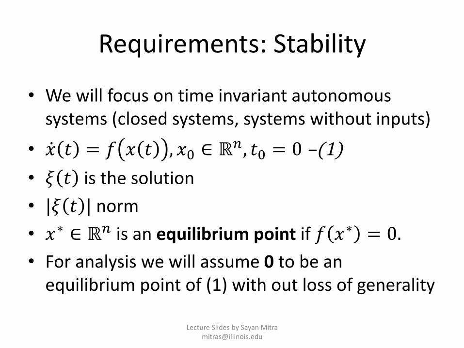
• Wewillfocusontimeinvariantautonomoussystems(closedsystems,systemswithoutinputs)
• �� 𝑡 = 𝑓 𝑥 𝑡 , 𝑥[ ∈ ℝ�, 𝑡[ = 0 –(1)• 𝜉 𝑡 isthesolution• |𝜉 𝑡 | norm• 𝑥∗ ∈ ℝ� isanequilibriumpointif𝑓 𝑥∗ = 0.• Foranalysiswewillassume0tobeanequilibriumpointof(1)withoutlossofgenerality

Example:PendulumPendulumequation𝑥M = 𝜃𝑥P = ��
𝑥P = ��M
��P = −𝑔𝑙 sin 𝑥M −
𝑘𝑚𝑥P
𝑥P𝑥M
= −ìísin 𝑥M −
Ê𝑥P
𝑥P
𝑘: frictioncoefficient
Twoequilibriumpoints: 0,0 , (𝜋, 0)
𝑙𝜃
𝑚
Lyapunov stability
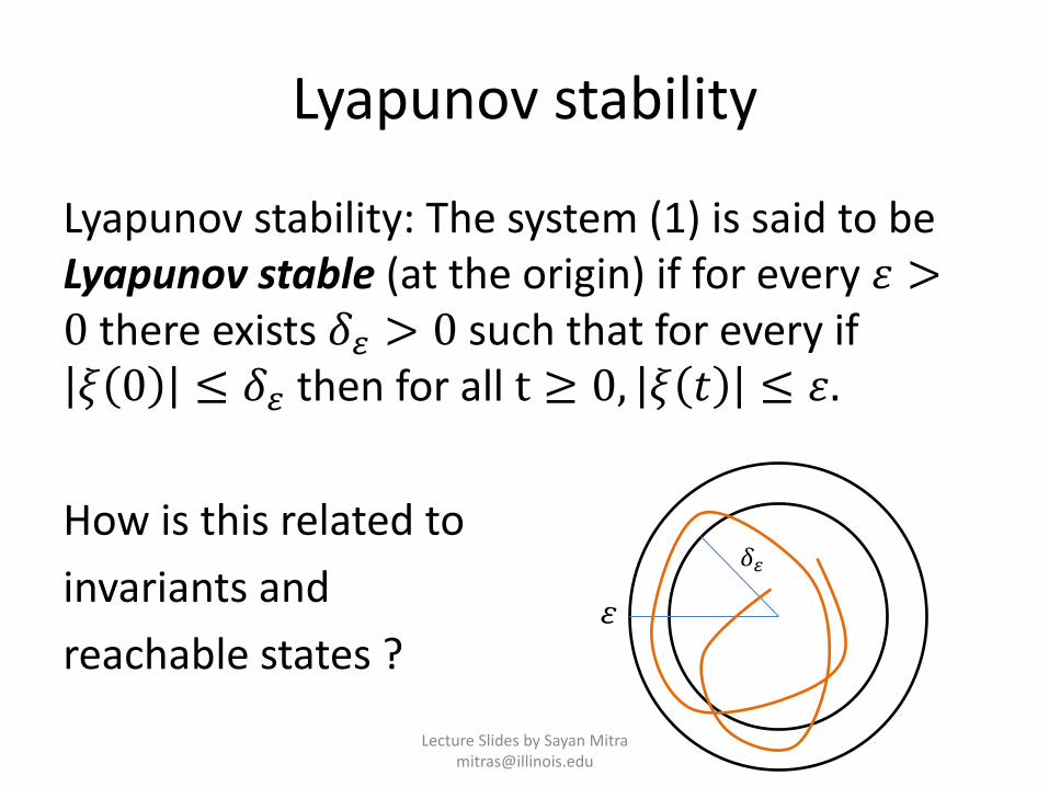
Lyapunov stability:Thesystem(1)issaidtobeLyapunov stable(attheorigin)ifforevery𝜀 >0thereexists𝛿ð > 0suchthatforeveryif𝜉 0 ≤ 𝛿ð thenforallt ≥ 0, 𝜉 𝑡 ≤ 𝜀.
Howisthisrelatedtoinvariantsandreachablestates?
𝛿ð

Asymptoticallystability
Thesystem(1)issaidtobeAsymptoticallystable(attheorigin)ifitisLyapunov stableandthereexists𝛿P > 0suchthatforeveryif 𝜉 0 ≤ 𝛿P thent → ∞, 𝜉 𝑡 → 𝟎.Ifthepropertyholdsforany𝛿P thenGloballyAsymptoticallyStable

Example:PendulumPendulumequation𝑥M = 𝜃𝑥P = ��
𝑥P = ��M
��P = −𝑔𝑙 sin 𝑥M −
𝑘𝑚𝑥P
𝑥P𝑥M
= −ìísin 𝑥M −
Ê𝑥P
𝑥P
Twoequilibriumpoints: 0,0 , (𝜋, 0)
𝒙 = 𝟎, 𝟎asymptoticallystable
𝒙 = 𝝅, 𝟎unstable
𝑥M
𝑥 P

Example:Pendulum
Pendulumequation
𝑥M = 𝜃𝑥P = ��
𝑥P = ��M
��P = −𝑔𝑙 sin 𝑥M −
𝑘𝑚 𝑥P
𝑥P𝑥M
= −ìísin 𝑥M −
Ê𝑥P
𝑥P
𝑘 = 0 nofriction𝒙∗ = 𝟎, 𝟎
stablebutnotasymptoticallystable
𝒙∗ = 𝝅, 𝟎unstable

Vanderpoloscillator
Vanderpoloscillator𝑑𝑥P
𝑑𝑡P − 𝜇 1 − 𝑥P𝑑𝑥𝑑𝑡 + 𝑥 = 0
𝑥M = 𝑥; 𝑥P = ��M;couplingcoefficient𝜇 = 20.1
𝑥P𝑥M
= 𝜇 1 − 𝑥MP 𝑥P −𝑥M𝑥P
stable?LectureSlidesbySayanMitra

Stabilityofsolutions*(insteadofpoints)
• Forany𝜉 ∈ PC ℝö[, ℝ� definethes-norm 𝜉 ÷ = sup»∈ℝ
| 𝜉 𝑡 |
• Adynamicalsystemcanbeseenasanoperatorthatmapsinitialstatestosignals𝑇:ℝ� → 𝑃𝐶 ℝö[, ℝ�
• Lyapunov stabilityrequiredthatthisoperatoriscontinuous
• Thesolution𝜉∗ isLyapunov stableif𝑇 iscontinuousas𝜉∗(0). i. e. ,forevery𝜀 > 0thereexists𝛿ð > 0suchthatforevery𝑥[ ∈ ℝ� if 𝜉∗ 0 − 𝑥[ ≤ 𝛿ð then 𝑇 𝜉∗ 𝑡 − 𝑇 𝑥[ ÷
≤ 𝜀.
*Notdiscussedinclass [email protected]

Butterfly*
𝑥P𝑥M
=2𝑥M𝑥P𝑥MP − 𝑥PP
Allsolutionsconvergeto0buttheequilibriumpoint(0,0)isnotLyapunov stable
*Notdiscussedinclass [email protected]
VerifyingStabilityforLinearSystems
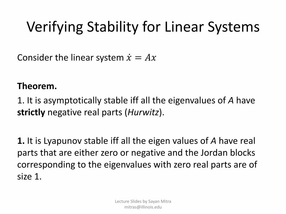
Considerthelinearsystem�� = 𝐴𝑥
Theorem.1.Itisasymptoticallystableiff alltheeigenvaluesofAhavestrictly negativerealparts(Hurwitz).
1.ItisLyapunov stableiff alltheeigen valuesofAhaverealpartsthatareeitherzeroornegativeandtheJordanblockscorrespondingtotheeigenvalueswithzerorealpartsareofsize1.
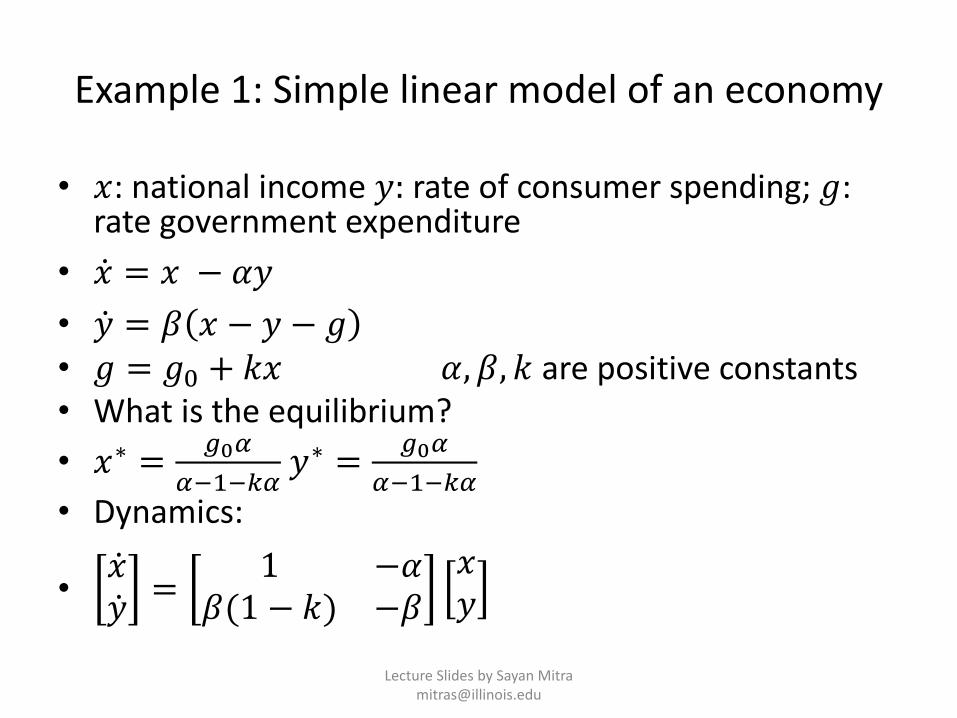
Example1:Simplelinearmodelofaneconomy
• 𝑥:nationalincome𝑦: rateofconsumerspending;𝑔:rategovernmentexpenditure
• �� = 𝑥 − 𝛼𝑦• �� = 𝛽 𝑥 − 𝑦 − 𝑔• 𝑔 = 𝑔[ + 𝑘𝑥 𝛼, 𝛽, 𝑘 arepositiveconstants• Whatistheequilibrium?• 𝑥∗ = ìáú
ú#M# ú𝑦∗ = ìáú
ú#M# ú• Dynamics:
• ���� = 1 −𝛼
𝛽(1 − 𝑘) −𝛽𝑥𝑦

Example:Simplelinearmodelofaneconomy
• 𝛼 = 3, 𝛽 = 1, 𝑘 = 0
• 𝜆M, 𝜆M∗ = (−.25 ± 𝑖1.714)
• Negativerealparts,therefore,asymptoticallystableandthenationalincomeandconsumerspendingrateconvergeto𝑥 = 1.764 𝑦 = 5.294

Stabilityofnonlinearsystems• Foranypositivedefinitefunctionofstate𝑉:ℝ� → ℝ– 𝑉 𝑥 ≥ 0 and𝑉 𝑥 = 0iff𝑥 = 0
• Sublevelsetsof𝐿þ = {𝑥 ∈ ℝ� |𝑉 𝑥 ≤ 𝑝}• 𝑉(𝜉 𝑡 )Vdifferentiablewithcontinuousfirstderivative
• �� = 𝑑 ÿ ! »Ç»
=?
• ßÿßÈ. ÇÇ»
𝜉 𝑡 = ßÿßÈ. 𝑓(𝑥) isalsocontinuous
• 𝑉 isradiallyunboundedif 𝑥 → ∞ ⇒ 𝑉 𝑥 → ∞
VerifyingStability
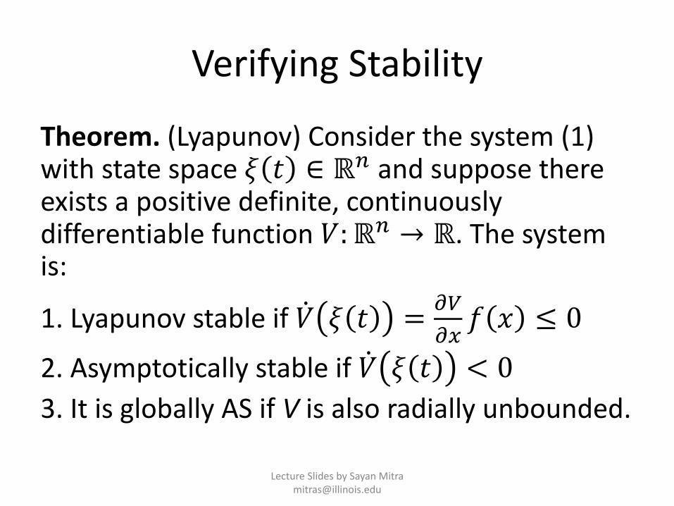
Theorem.(Lyapunov)Considerthesystem(1)withstatespace𝜉 𝑡 ∈ ℝ� andsupposethereexistsapositivedefinite,continuouslydifferentiablefunction𝑉:ℝ� → ℝ.Thesystemis:
1.Lyapunov stableif�� 𝜉 𝑡 = ßÿßÈ𝑓 𝑥 ≤ 0
2.Asymptoticallystableif�� 𝜉 𝑡 < 03.ItisgloballyASifVisalsoradiallyunbounded.

Proofsketch:Lyapunovstableif�� ≤ 0
• Assume�� ≤ 0• ConsideraballBðaroundtheoriginof
radius𝜀 > 0.• Pickapositivenumber𝑏 < min
È Zð𝑉 𝑥 .
• Let𝛿 bearadiusofballaroundoriginwhichisinsideB$ = 𝑥 𝑉 𝑥 ≤ 𝑏}
• SincealongalltrajectoriesVisnon-increasing,startingfrom𝐵$ eachsolutionsatisfies𝑉 𝜉 𝑡 ≤ 𝑏andthereforeremainsinBð
Bð𝐿% 𝐵$

Proofsketch:Asymptoticallystableif�� 𝜉 𝑡 < 0
• Assume�� < 0• Takearbitrary 𝜉 0 ≤ 𝛿,wherethis𝛿
comesfromsome𝜀 forLyapunov stability• Since𝑉 𝜉 . > 0 anddecreasingalong𝜉it
hasalimit𝑐 ≥ 0at𝑡 → ∞• Itsufficestoshowthatthislimitisactually0• Supposenot,c>0thenthesolutionevolves
inthecompactset𝑆 = 𝑥 𝑟 ≤ 𝑥 ≤ 𝜀} forsomesufficientlysmall𝑟
• Let𝑑 = maxÈ∈&
��(𝑥) [slowestrate]• Thisnumberiswell-definedandnegative• �� 𝜉 𝑡 ≤ 𝑑forallt• 𝑉 𝑡 ≤ 𝑉 0 + 𝑑𝑡• Buttheneventually𝑉 𝑡 < 𝑐
Bð
𝑟

Example2
• ��M = −𝑥M + 𝑔 𝑥P ; ��P = −𝑥P + ℎ 𝑥M
• 𝑔 𝑢 ≤ 'P, ℎ 𝑢 ≤ '
P
• Use𝑉 = MP𝑥MP + 𝑥PP ≥ 0
• �� = 𝑥M��M + 𝑥P��P=−𝑥MP −𝑥PP +𝑥M𝑔 𝑥P + 𝑥Pℎ 𝑥M≤ −𝑥MP −𝑥PP +
MP|𝑥M𝑥P| + |𝑥P𝑥M|
≤ − MP(𝑥MP + 𝑥PP) = −𝑉
Weconcludeglobalasymptoticstability(infactglobalexponentialstability)withoutknowingsolutions
𝑥M − 𝑥PP≥ 0
𝑥MP + 𝑥PP ≥ 2 𝑥M𝑥P
𝑥M𝑥P ≤12 (𝑥M
P + 𝑥PP)

Proposition. EverysublevelsetofVisaninvariant
Proof.𝑉 𝜉 𝑡 == 𝑉 𝜉 0 + ∫ �� 𝜉 𝜏 𝑑𝜏»
[≤ 𝑉(𝜉(0))

Anaside:Checkinginductiveinvariants
• 𝑨 = 𝑋,𝑄[, 𝑇– 𝑋: setofvariables– 𝑄[ ⊆ 𝑣𝑎𝑙 𝑋– 𝑇 ⊆ 𝑣𝑎𝑙 𝑋 ×𝑣𝑎𝑙 𝑋 writtenasaprogram𝑥′ ⊆ 𝑇(𝑥)
• Howdowecheckthat𝐼 ⊆ 𝑣𝑎𝑙(𝑋) isaninductiveinvariant?– 𝑄[ ⇒ 𝐼(𝑋)– 𝐼 𝑋 ⇒ 𝐼(𝑇 𝑋 )
• Impliesthat𝑅𝑒𝑎𝑐ℎ𝑨 𝑄[ ⊆ 𝐼withoutcomputingtheexecutionsorreachablestatesofA
• Thekeyistofindsuch𝐼LectureSlidesbySayanMitra

FindingLyapunov Functions
• ThekeytousingLyapunov theoryistofindaLyapunov functionandverifythatithastheproperties
• Ingeneralfornonlinearsystemsthisishard• Thereareseveralapproaches– LinearquadraticLyapunov functionsforlinearsystems– Decidetheform/templateofthefunction(e.g.,quadratic),parameterizedbysomeparameters
– Trytofindvaluesoftheparameterssothattheconditionshold
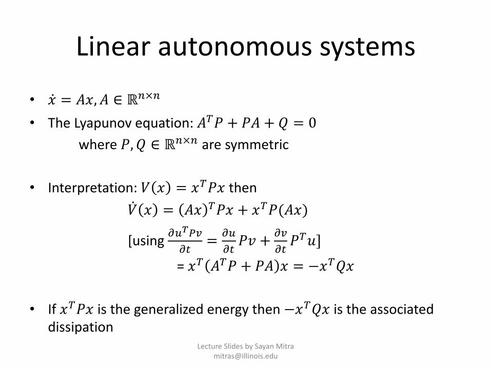
Linearautonomoussystems
• �� = 𝐴𝑥, 𝐴 ∈ ℝ�×�
• TheLyapunov equation:𝐴)𝑃 + 𝑃𝐴 + 𝑄 = 0where𝑃, 𝑄 ∈ ℝ�×� aresymmetric
• Interpretation:𝑉 𝑥 = 𝑥)𝑃𝑥 then�� 𝑥 = 𝐴𝑥 )𝑃𝑥 + 𝑥)𝑃(𝐴𝑥)
[usingß'*�+ß»
= ß'ß»𝑃𝑣 + ß+
ß»𝑃)𝑢]
=𝑥) 𝐴)𝑃 + 𝑃𝐴 𝑥 = −𝑥)𝑄𝑥
• If𝑥)𝑃𝑥 isthegeneralizedenergythen−𝑥)𝑄𝑥 istheassociateddissipation

QuadraticLyapunov Functions
• If𝑃 > 0 (positivedefinite)• 𝑉 𝑥 = 𝑥)𝑃𝑥 = 0 ⇔ 𝑥 = 0• Thesub-levelsetsareellipsoids• If𝑄 > 0 thenthesystemisgloballyasymptoticallystable

SameexampleLyapunovequationsaresolvedasasetof� ��M
Pequationsin
𝑛 𝑛 + 1 /2 variables.CostO(𝑛,)
Choose𝑄 = 1 00 1 solving
Lyapunov equationsweget𝑃 = 2.59 −2.29−2.29 4.92 andwegetthe
quadraticLyapunov function𝑥 − 𝑥∗ 𝑃 𝑥 − 𝑥∗ ) anasequenceofinvariants

ConverseLyapunov
ConverseLyapunov theoremsshowthatconditionsoftheprevioustheoremarealsonecessary.Forexample,ifthesystemisasymptoticallystablethenthereexistsapositivedefinite,continuouslydifferentiablefunctionV,thatsatisfiestheinequalities.
ForexampleiftheLTIsystem�� = 𝐴𝑥 isgloballyasymptoticallystablethenthereisaquadraticLyapunov functionthatprovesit.


![Logics of Dynamical Systems - cs.cmu.eduaplatzer/pub/lds-lics.pdf · ical systems described by differential equations [44], and hybrid dynamical systems alias hybrid systems combining](https://static.documents.pub/doc/80x56/5f06b1f57e708231d4194613/logics-of-dynamical-systems-cscmu-aplatzerpublds-licspdf-ical-systems-described.jpg)


