Lecture 4 Knowledge-Based Systems IS430mzali/courses/Fall14/Cis330/slides/Handouts2... ·...

Lecture 2: Slide 1

Knowledge-Based SystemsIS430

Mostafa Z. [email protected]

Lecture 4

Fall 2009

Fundamental Simulation Concepts

Slide 2 of 46

What We’ll Do ...

• Underlying ideas, methods, and issues in simulation

• Software-independent (setting up for Arena)• Centered around an example of a simple

processing systemDecompose the problemTerminologySimulation by handSome basic statistical issuesOverview of a simulation study

Slide 3 of 46

The System:A Simple Processing System

ArrivingBlank Parts

DepartingFinished Parts

Machine(Server)

Queue (FIFO) Part in Service

4567

• General intent:Estimate expected productionWaiting time in queue, queue length, proportion of time machine is busy

• Time unitsCan use different units in different places … must declareBe careful to check the units when specifying inputsDeclare base time units for internal calculations, outputsBe reasonable (interpretation, roundoff error)

Slide 4 of 46

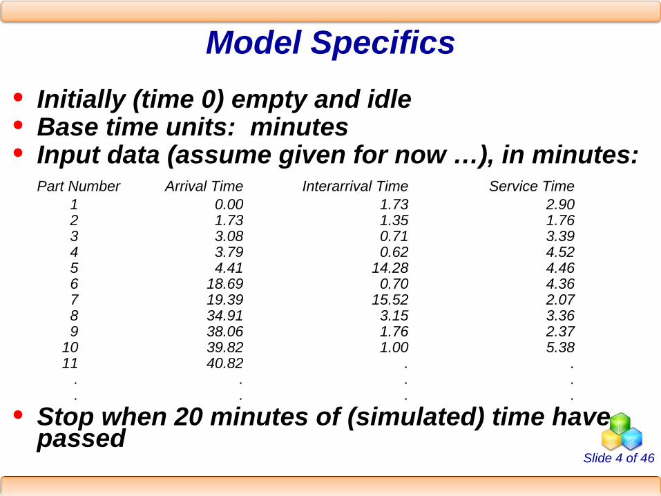
Model Specifics• Initially (time 0) empty and idle• Base time units: minutes• Input data (assume given for now …), in minutes:

Part Number Arrival Time Interarrival Time Service Time1 0.00 1.73 2.902 1.73 1.35 1.763 3.08 0.71 3.394 3.79 0.62 4.525 4.41 14.28 4.466 18.69 0.70 4.367 19.39 15.52 2.078 34.91 3.15 3.369 38.06 1.76 2.37

10 39.82 1.00 5.3811 40.82 . .

. . . .

. . . .

• Stop when 20 minutes of (simulated) time have passed

Slide 5 of 46

Goals of the Study:Output Performance Measures

• Total production of parts over the run (P)• Average waiting time of parts in queue:

• Maximum waiting time of parts in queue:

N = no. of parts completing queue waitWQi = waiting time in queue of ith partKnow: WQ1 = 0 (why?)

N > 1 (why?)N

WQN

ii∑

=1

iNi

WQmax,...,1=

Slide 6 of 46

Goals of the Study:Output Performance Measures (cont’d.)

• Time-average number of parts in queue:

• Maximum number of parts in queue:• Average and maximum total time in system of

parts (a.k.a. cycle time):

Q(t) = number of parts in queueat time t20

)(200∫ dttQ

)(max200

tQt≤≤

iPi

P

ii

TSP

TSmax

,...,11 ,

=

=∑

TSi = time in system of part i

Slide 7 of 46

Goals of the Study:Output Performance Measures (cont’d.)

• Utilization of the machine (proportion of time busy)

• Many others possible (information overload?)

⎩⎨⎧

=∫tt

tBdttB

timeat idle is machine the if0 timeat busy is machine the if1

)(,20

)(200

Slide 8 of 46

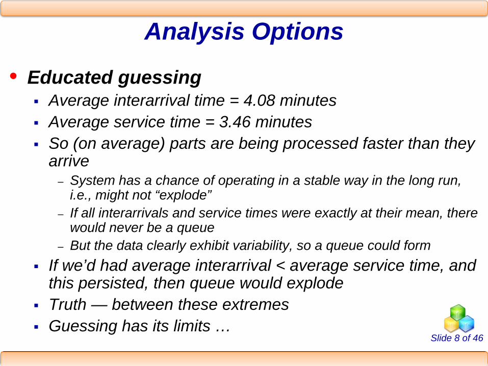
Analysis Options

• Educated guessingAverage interarrival time = 4.08 minutesAverage service time = 3.46 minutesSo (on average) parts are being processed faster than they arrive

– System has a chance of operating in a stable way in the long run, i.e., might not “explode”

– If all interarrivals and service times were exactly at their mean, there would never be a queue

– But the data clearly exhibit variability, so a queue could formIf we’d had average interarrival < average service time, and this persisted, then queue would explodeTruth — between these extremesGuessing has its limits …

Slide 9 of 46

Analysis Options (cont’d.)

• Queueing theoryRequires additional assumptions about the modelPopular, simple model: M/M/1 queue

– Interarrival times ~ exponential– Service times ~ exponential, indep. of interarrivals– Must have E(service) < E(interarrival)– Steady-state (long-run, forever)– Exact analytic results; e.g., average waiting time in queue is

Problems: validity, estimating means, time frameOften useful as first-cut approximation

time) E(service time) ivalE(interarr 2

==

− S

A

SA

Sμμ

μμμ ,

Slide 10 of 46

Mechanistic Simulation

• Individual operations (arrivals, service times) will occur exactly as in reality

• Movements, changes occur at the right “time,” in the right order

• Different pieces interact• Install “observers” to get output performance

measures• Concrete, “brute-force” analysis approach• Nothing mysterious or subtle

But a lot of details, bookkeepingSimulation software keeps track of things for you

Mostafa Ali

Sticky Note

traversing the search space of possible keys

Slide 11 of 46

Pieces of a Simulation Model

• Entities“Players” that move around, change status, affect and are affected by other entitiesDynamic objects — get created, move around, leave (maybe)Usually represent “real” things

– Our model: entities are the partsCan have “fake” entities for modeling “tricks”

– Breakdown demon, break angelThough Arena has built-in ways to model these examples directly

Usually have multiple realizations floating aroundCan have different types of entities concurrentlyUsually, identifying the types of entities is the first thing to do in building a model

Slide 12 of 46

Pieces of a Simulation Model (cont’d.)

• AttributesCharacteristic of all entities: describe, differentiateAll entities have same attribute “slots” but different values for different entities, for example:

– Time of arrival– Due date– Priority– Color

Attribute value tied to a specific entityLike “local” (to entities) variablesSome automatic in Arena, some you define

Slide 13 of 46


• (Global) VariablesReflects a characteristic of the whole model, not of specific entitiesUsed for many different kinds of things

– Travel time between all station pairs– Number of parts in system– Simulation clock (built-in Arena variable)

Name, value of which there’s only one copy for the whole modelNot tied to entitiesEntities can access, change variablesWriting on the wall (rewriteable)Some built-in by Arena, you can define others

Slide 14 of 46


• ResourcesWhat entities compete for

– People– Equipment– Space

Entity seizes a resource, uses it, releases itThink of a resource being assigned to an entity, rather than an entity “belonging to” a resource“A” resource can have several units of capacity

– Seats at a table in a restaurant– Identical ticketing agents at an airline counter

Number of units of resource can be changed during the simulation

Slide 15 of 46


• QueuesPlace for entities to wait when they can’t move on (maybe since the resource they want to seize is not available)Have names, often tied to a corresponding resourceCan have a finite capacity to model limited space — have to model what to do if an entity shows up to a queue that’s already fullUsually watch the length of a queue, waiting time in it

Slide 16 of 46


• Statistical accumulatorsVariables that “watch” what’s happeningDepend on output performance measures desired“Passive” in model — don’t participate, just watchMany are automatic in Arena, but some you may have to set up and maintain during the simulationAt end of simulation, used to compute final output performance measures

Slide 17 of 46


• Statistical accumulators for the simple processing system

Number of parts produced so farTotal of the waiting times spent in queue so farNo. of parts that have gone through the queueMax time in queue we’ve seen so farTotal of times spent in systemMax time in system we’ve seen so farArea so far under queue-length curve Q(t)Max of Q(t) so farArea so far under server-busy curve B(t)

Slide 18 of 46

Simulation Dynamics:The Event-Scheduling “World View”

• Identify characteristic events• Decide on logic for each type of event to

Effect state changes for each event typeObserve statisticsUpdate times of future events (maybe of this type, other types)

• Keep a simulation clock, future event calendar• Jump from one event to the next, process,

observe statistics, update event calendar• Must specify an appropriate stopping rule• Usually done with general-purpose programming

language (C, FORTRAN, etc.)

Slide 19 of 46

Events for theSimple Processing System

• Arrival of a new part to the systemUpdate time-persistent statistical accumulators (from last event to now)

– Area under Q(t)– Max of Q(t)– Area under B(t)

“Mark” arriving part with current time (use later)If machine is idle:

– Start processing (schedule departure), Make machine busy, Tally waiting time in queue (0)

Else (machine is busy):– Put part at end of queue, increase queue-length variable

Schedule the next arrival event

Slide 20 of 46

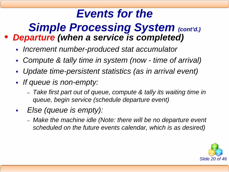
Events for theSimple Processing System (cont’d.)

• Departure (when a service is completed)Increment number-produced stat accumulatorCompute & tally time in system (now - time of arrival)Update time-persistent statistics (as in arrival event)If queue is non-empty:

– Take first part out of queue, compute & tally its waiting time in queue, begin service (schedule departure event)

Else (queue is empty):– Make the machine idle (Note: there will be no departure event

scheduled on the future events calendar, which is as desired)

Slide 21 of 46

Events for theSimple Processing System (cont’d.)

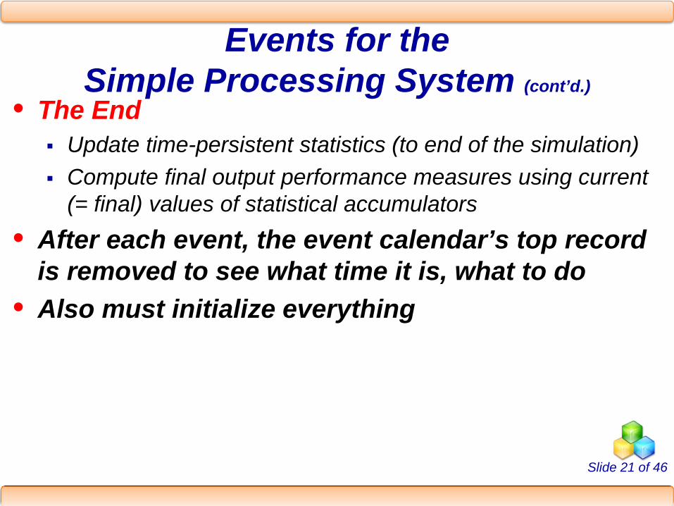
• The EndUpdate time-persistent statistics (to end of the simulation)Compute final output performance measures using current (= final) values of statistical accumulators

• After each event, the event calendar’s top record is removed to see what time it is, what to do

• Also must initialize everything

Slide 22 of 46

Some Additional Specifics for theSimple Processing System

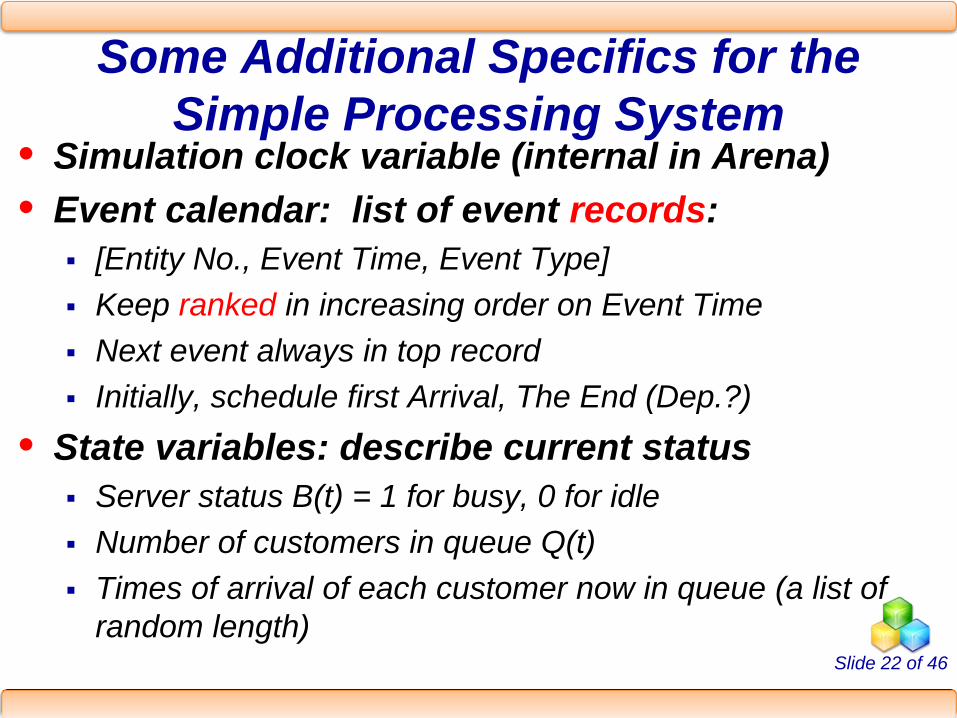
• Simulation clock variable (internal in Arena)• Event calendar: list of event records:

[Entity No., Event Time, Event Type]Keep ranked in increasing order on Event TimeNext event always in top recordInitially, schedule first Arrival, The End (Dep.?)

• State variables: describe current statusServer status B(t) = 1 for busy, 0 for idleNumber of customers in queue Q(t)Times of arrival of each customer now in queue (a list of random length)

Slide 23 of 46

Simulation by Hand

• Manually track state variables, statistical accumulators

• Use “given” interarrival, service times• Keep track of event calendar• “Lurch” clock from one event to the next• Will omit times in system, “max” computations

here (see text for complete details)

Slide 24 of 46

System

Clock

B(t)

Q(t)

Arrival times of custs. in queue

Event calendar

Number of completed waiting times in queue

Total of waiting times in queue

Area under Q(t)

Area under B(t)

Q(t) graph B(t) graph

Time (Minutes) Interarrival times 1.73, 1.35, 0.71, 0.62, 14.28, 0.70, 15.52, 3.15, 1.76, 1.00, ... Service times 2.90, 1.76, 3.39, 4.52, 4.46, 4.36, 2.07, 3.36, 2.37, 5.38, ...

Simulation by Hand:Setup

01

23

4

0 5 10 15 20

012

0 5 10 15 20

Slide 25 of 46

System

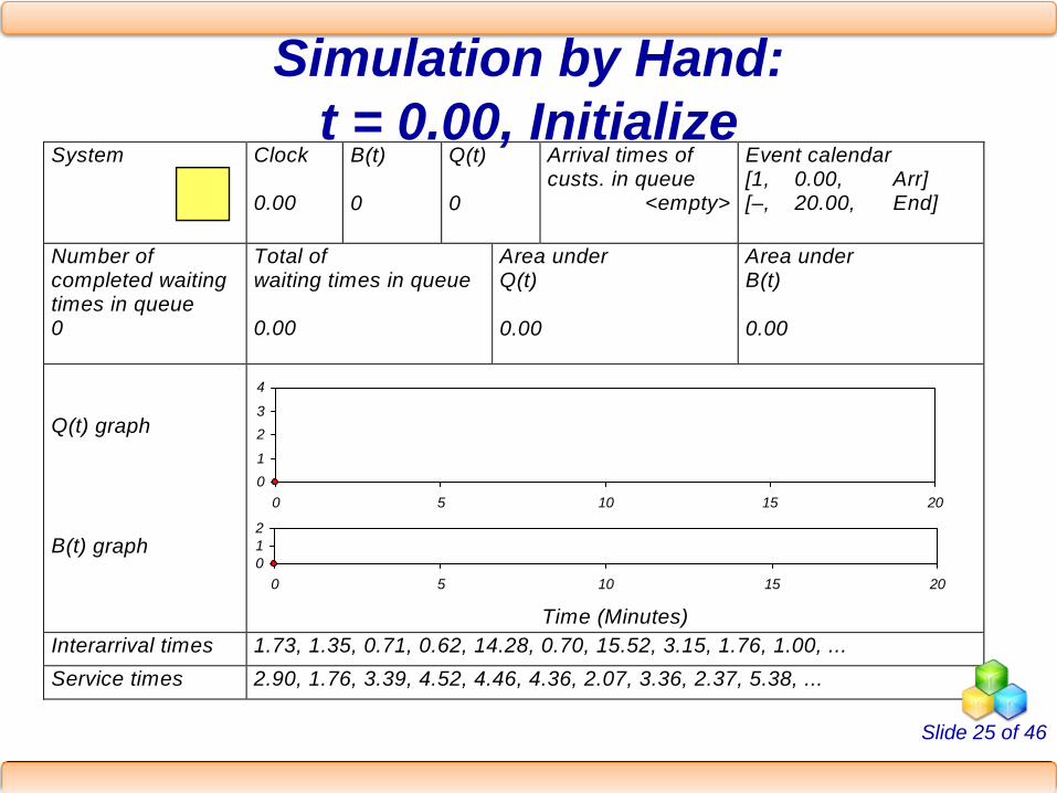
Clock 0.00

B(t) 0

Q(t) 0


<empty>

Event calendar [1, 0.00, Arr] [–, 20.00, End]

Number of completed waiting times in queue 0

Total of waiting times in queue 0.00

Area under Q(t) 0.00

Area under B(t) 0.00



Simulation by Hand:t = 0.00, Initialize

01

23

4

0 5 10 15 20

012

0 5 10 15 20

Slide 26 of 46

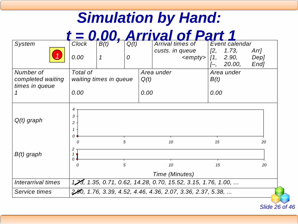
System

Clock 0.00

B(t) 1

Q(t) 0


<empty>

Event calendar [2, 1.73, Arr] [1, 2.90, Dep] [–, 20.00, End]







Simulation by Hand:t = 0.00, Arrival of Part 1

01

23

4

0 5 10 15 20

012

0 5 10 15 20

1

Slide 27 of 46

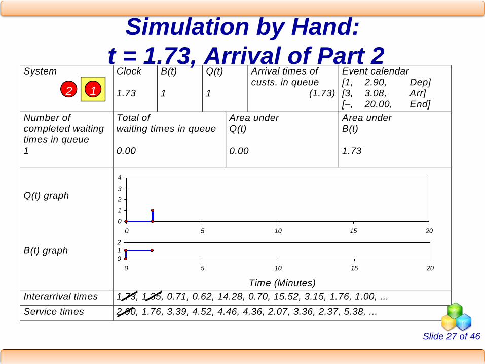
System

Clock 1.73

B(t) 1

Q(t) 1


(1.73)

Event calendar [1, 2.90, Dep] [3, 3.08, Arr] [–, 20.00, End]








01

23

4

0 5 10 15 20

012

0 5 10 15 20

12

Slide 28 of 46

System

Clock 2.90

B(t) 1

Q(t) 0


<empty>








Simulation by Hand:t = 2.90, Departure of Part 1

01

23

4

0 5 10 15 20

012

0 5 10 15 20

2

Slide 29 of 46

System

Clock 3.08

B(t) 1

Q(t) 1


(3.08)









01

23

4

0 5 10 15 20

012

0 5 10 15 20

23

Slide 30 of 46

System

Clock 3.79

B(t) 1

Q(t) 2


(3.79, 3.08)









01

23

4

0 5 10 15 20

012

0 5 10 15 20

234

Slide 31 of 46

System

Clock 4.41

B(t) 1

Q(t) 3


(4.41, 3.79, 3.08)









01

23

4

0 5 10 15 20

012

0 5 10 15 20

2345

Slide 32 of 46

System

Clock 4.66

B(t) 1

Q(t) 2


(4.41, 3.79)









01

23

4

0 5 10 15 20

012

0 5 10 15 20

345

Slide 33 of 46

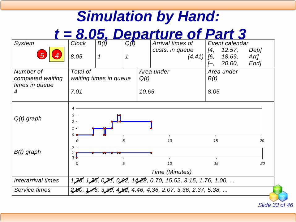
System

Clock 8.05

B(t) 1

Q(t) 1


(4.41)









01

23

4

0 5 10 15 20

012

0 5 10 15 20

45

Slide 34 of 46

System

Clock 12.57

B(t) 1

Q(t) 0


()









01

23

4

0 5 10 15 20

012

0 5 10 15 20

5

Slide 35 of 46

System

Clock 17.03

B(t) 0

Q(t) 0

Arrival times of custs. in queue ()

Event calendar [6, 18.69, Arr] [–, 20.00, End]








01

23

4

0 5 10 15 20

012

0 5 10 15 20

Slide 36 of 46

System

Clock 18.69

B(t) 1

Q(t) 0

Arrival times of custs. in queue ()

Event calendar [7, 19.39, Arr] [–, 20.00, End] [6, 23.05, Dep]








01

23

4

0 5 10 15 20

012

0 5 10 15 20

6

Slide 37 of 46

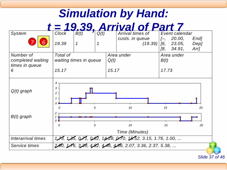
System

Clock 19.39

B(t) 1

Q(t) 1


(19.39)

Event calendar [–, 20.00, End] [6, 23.05, Dep] [8, 34.91, Arr]








01

23

4

0 5 10 15 20

012

0 5 10 15 20

67

Slide 38 of 46

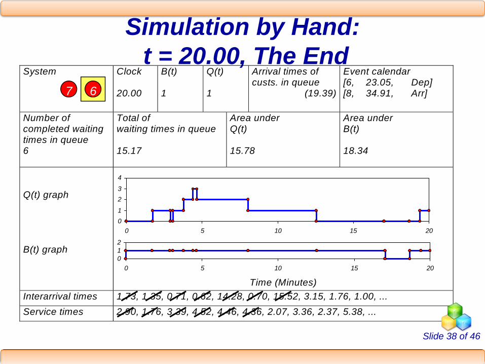
Simulation by Hand:t = 20.00, The End

01

23

4

0 5 10 15 20

012

0 5 10 15 20

67

System

Clock 20.00

B(t) 1

Q(t) 1


(19.39)

Event calendar [6, 23.05, Dep] [8, 34.91, Arr]







Slide 39 of 46

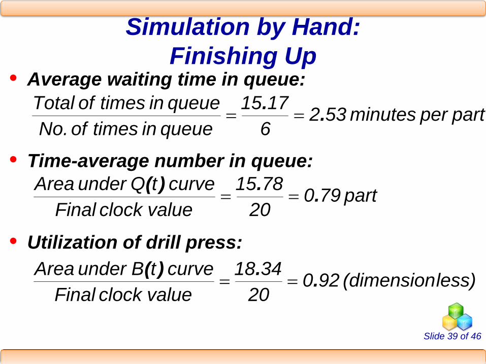
Simulation by Hand:Finishing Up

• Average waiting time in queue:

• Time-average number in queue:

• Utilization of drill press:

part per minutes 53261715

queue in times of No.queueintimes of Total .. ==

part 79020

7815valueclock Final

curve under Area ..)( ==tQ

less)(dimension 92020

3418valueclock Final

curve under Area ..)( ==tB

Slide 40 of 46

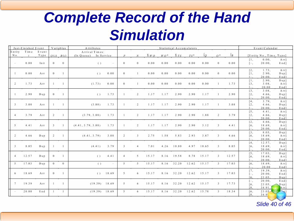
Complete Record of the Hand Simulation

Slide 41 of 46

Event-Scheduling Logic via Programming

• Clearly well suited to standard programming language

• Often use “utility” libraries for:List processingRandom-number generationRandom-variate generationStatistics collectionEvent-list and clock managementSummary and output

• Main program ties it together, executes events in order

Slide 42 of 46

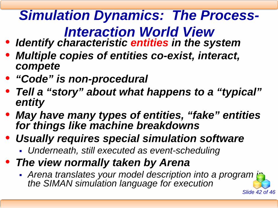
Simulation Dynamics: The Process-Interaction World View

• Identify characteristic entities in the system• Multiple copies of entities co-exist, interact,

compete• “Code” is non-procedural• Tell a “story” about what happens to a “typical”

entity• May have many types of entities, “fake” entities

for things like machine breakdowns• Usually requires special simulation software

Underneath, still executed as event-scheduling• The view normally taken by Arena

Arena translates your model description into a program in the SIMAN simulation language for execution

Slide 43 of 46

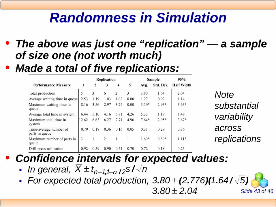
Randomness in Simulation

• The above was just one “replication” — a sample of size one (not worth much)

• Made a total of five replications:

• Confidence intervals for expected values:In general, For expected total production,

nstX n //, 211 α−−±)/.)(.(. 56417762803 ±

042803 .. ±

Notesubstantialvariabilityacrossreplications

Slide 44 of 46

Comparing Alternatives

• Usually, simulation is used for more than just a single model “configuration”

• Often want to compare alternatives, select or search for the best (via some criterion)

• Simple processing system: What would happen if the arrival rate were to double?

Cut interarrival times in halfRerun the model for double-time arrivalsMake five replications

Slide 45 of 46

Results: Original vs. Double-Time Arrivals

• Original – circles• Double-time – triangles• Replication 1 – filled in• Replications 2-5 – hollow• Note variability• Danger of making

decisions based on one (first) replication

• Hard to see if there are really differences

• Need: Statistical analysis of simulation output data

Slide 46 of 46

Overview of a Simulation Study

• Understand the system• Be clear about the goals• Formulate the model representation• Translate into modeling software• Verify “program”• Validate model• Design experiments• Make runs• Analyze, get insight, document results

Date post:	27-Mar-2018
Category:	Documents
Upload:	danghanh
View:	219 times
Download:	3 times

Lecture 4 Knowledge-Based Systems IS430mzali/courses/Fall14/Cis330/slides/Handouts2... ·...

Documents