Lecture 4 - Transverse Optics II · Lecture 4 - E. Wilson - 22 Oct 2010 –-Slide2 Contents of...

Lecture 4 - E. Wilson - 22 Oct 2010 –- Slide 1

Lecture 4 - Transverse Optics II

ACCELERATOR PHYSICS

MT 2010

E. J. N. Wilson


Contents of previous lecture -Transverse Optics I

Transverse coordinatesVertical FocusingCosmotronWeak focusing in a synchrotron The “n-value”Gutter Transverse ellipseCosmotron peopleAlternating gradients Equation of motion in transverse co-

ordinates


Lecture 4 - Transverse Optics II Contents

Equation of motion in transverse co-ordinates

Check Solution of Hill Twiss Matrix Solving for a ring The lattice Beam sections Physical meaning of Q and beta Smooth approximation


Relativistic H of a charged particle in an electromagnetic field

Remember from special relativity:

i.e. the energy of a free particle

Add in the electromagnetic field» electrostatic energy» magnetic vector potential has same dimensions

as momentum

px =mvx

1− β2 , x

py =mvy

1− β 2 , y

pz =mvz

1− β 2 , z

H = px2c2 + py

2c2 + pz2c2 + m0

2c4

eφeA

H q,p,t( ) = eφ + c p − eA( )2 + m02c4[ ]

12


Hamiltonian for a particle in an accelerator

Note this is not independent of q because

Montague (pp 39 – 48) does a lot of rigorous, clever but confusing things but in the end he just turns H inside out

is the new Hamiltonian with s as the independent variable instead of t (see M 48)

Wilson obtains

» assumes curvature is small» assumes» assumes magnet has no ends» assumes small angles» ignores y plane

Dividing by

Finally (W Equ 8)

A = A x, y, s( )

ps

φ = 0 Ax = Ay = 0px << ps

H =

px2

2− eAs

P = px2 + py

2 + pz2

H =

p2

2−

eP

As =′ x ( )2

2−

As

Bρ( )

H q,p,t( ) = eφ + c p − eA( )2 + m02c4[ ]

12


Multipoles in the Hamiltonian

We said contains x (and y) dependance

We find out how by comparing the two expressions:

We find a series of multipoles:

For a quadrupole n=2 and:

H =

′ x ( )2

2−

As

Bρ( )As

As = Ann∑ xn

H =

′ x ( )2

2+

k(s)x2

2

By ( y= 0)= −

∂As

∂x= − nAnn∑ xn−1

By ( y= 0)=

1(n −1)!

∂ (n −1)By

∂x(n−1) xn −1

H =

′ x ( )2

2+

1Bρ( )n

∑ 1n!

∂ (n −1)By

∂x(n −1) xn


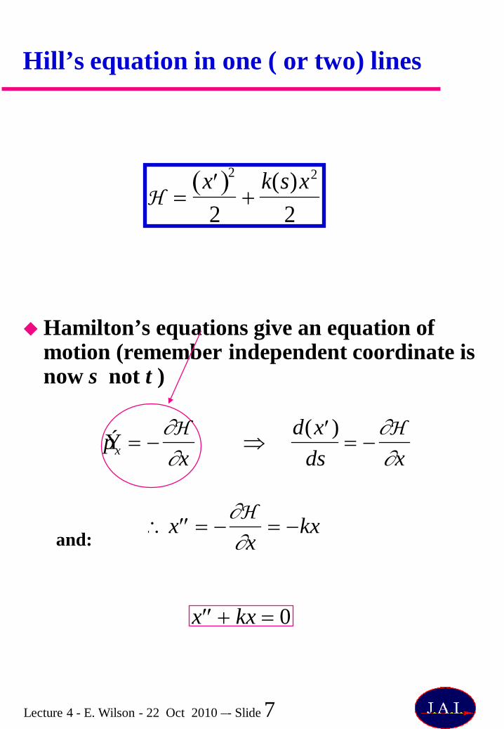
Hill’s equation in one ( or two) lines

Hamilton’s equations give an equation of motion (remember independent coordinate is now s not t )

and:

′ ′ x + kx = 0

Ý p x = −

∂H∂x

⇒ d( ′ x )

ds= −

∂H∂x

∴ ′ ′ x = −

∂H∂x

= −kx

H =

′ x ( )2

2+

k(s)x2

2


Other interesting forms

H =

p2

2+

k s( ) x2

2

H =

px2

2+

1Be( )n=0

∞

∑ 1n!

∂ n −1( )Bz∂x n −1( )

xn

eAsp

=1Be

1n!

∂ n −1( )Bz∂x n −1( )

x n∑

H ≈ −

eAsp

+p x

2

2

H ≈ −

eAsp

− 1− p x2( )1/ 2

In x plane

Small divergences:

Substitute a Taylor series:

Multipoles each have a term:

Bz z = 0( ) =

∂As∂x

= n An x n−1( )

Quadrupoles:

But:



Hill’s equation (linear-periodic coefficients)

– where at quadrupoles

– like restoring constant in harmonic motion Solution (e.g. Horizontal plane)

Condition

Property of machine Property of the particle (beam) ε Physical meaning (H or V planes)

EnvelopeMaximum excursions

k = − 1

Bρ( )dBzdx

β s( ) ϕ = ds

β s( )∫

y = εβ s( ) ′ ˆ y = ε / β s( )

ε β s( )

y = β s( ) ε sin φ s( ) + φ0[ ]

d 2 yds 2 + k s( )y = 0


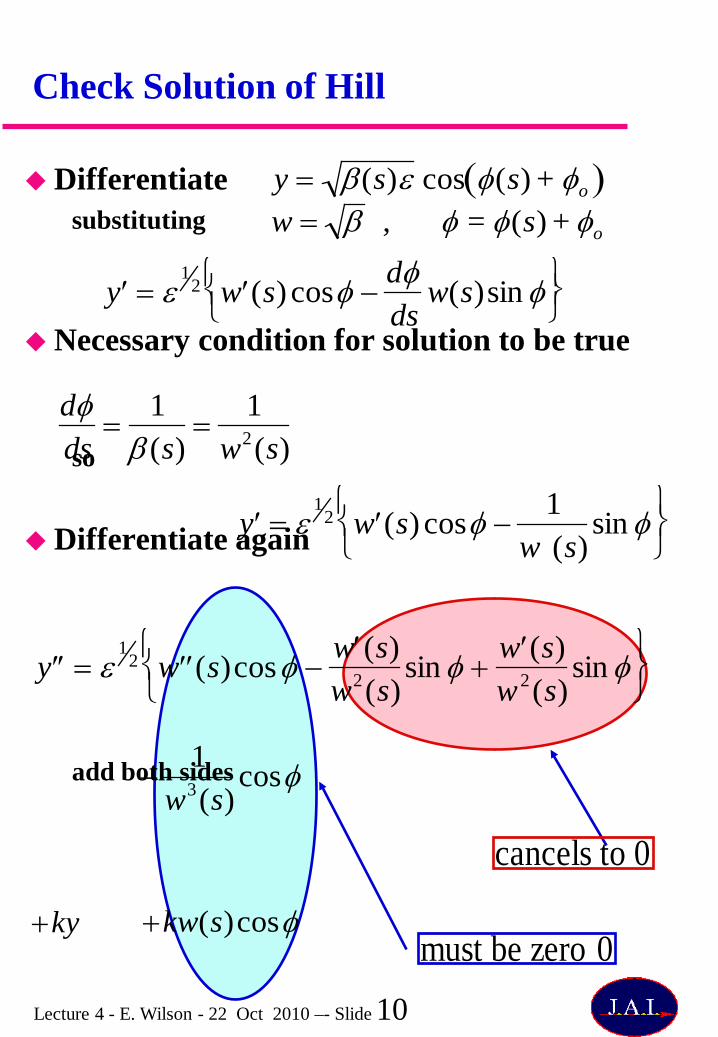
Check Solution of Hill

Differentiatesubstituting

Necessary condition for solution to be true

so

Differentiate again

add both sides

w = β , φ = φ(s) + φo

′ y = ε1

2 ′ w (s) cosφ −dφds

w(s)sin φ

dφds

=1

β (s)=

1w2(s)

′ y = ε1

2 ′ w (s) cosφ −1

w (s)sin φ

′ ′ y = ε1

2 ′ ′ w (s)cosφ −′ w (s)

w2(s)sin φ +

′ w (s)w2(s)

sin φ

−1

w3(s)cosφ

+ky +kw(s)cosφ

cancels to 0

must be zero 0

y = β(s)ε cos φ(s) + φo( )


Continue checking

The condition that these three coefficientssum to zero is a differential equation for the envelope

′ ′ y = ε1

2 ′ ′ w (s)cosφ −′ w (s)

w2(s)sin φ +

′ w (s)w2(s)

sin φ

−1

w3(s)cosφ

+ky +kw(s)cosφ

cancels to 0

must be zero 0

′ ′ w (s) + kw(s) −1

w3(s)= 0

12

β ′ ′ β −14

′ β 2 + kβ 2 = 1

alternatively


All such linear motion from points 1 to 2 can be described by a matrix like:

To find elements first use notationWe knowDifferentiate and remember

Trace two rays one starts “cosine” The other starts with “sine”We just plug in the “c” and “s” expression

for displacement an divergence at point 1 and the general solutions at point 2 on LHS

Matrix then yields four simultaneous equations with unknowns : a b c d which can be solved

y'= ε1/2w' cos ϕ + φ0( ) −

εw

1/2sin ϕ + φ0( )

Twiss Matrix

y s2( )y' s2( )

=

a bc d

y s1( )y' s1( )

= M12

y s1( )y' s1( )

.

w = β

y = ε1/2w cos ϕ + φ0( )

ϕ =

1β

=1

w2

φ = 0φ = π / 2


Twiss Matrix (continued)

Writing The matrix elements are

Above is the general case but to simplify we consider points which are separated by only one PERIOD and for which

The “period” matrix is then

If you have difficulty with the concept of a period just think of a single turn.

φ = φ2 − φ1

M12 =

w2w1

cos ϕ − w2w1' sin ϕ , w1w2 sin ϕ

−1 + w1w1

' w2w2'

w1w2 sin ϕ −

w1'

w2−

w2'

w1

cos ϕ , w1

w2 cos ϕ + w1w2

' sin ϕ

w1 = w2 = w , ′ w 1 = ′ w 2 = ′ w , µ = φ2 − φ1 = 2πQ

M = cos µ − ww ' sin µ , w2 sin µ

−1 + w2w '2

w2 sin µ , cos µ + ww' sin µ


Twiss concluded

Can be simplified if we define the “Twiss” parameters:

Giving the matrix for a ring (or period)

M = cos µ − ww ' sin µ , w2 sin µ

−1 + w2w '2

w2 sin µ , cos µ + ww' sin µ

β = w2 , α = −12

′ β , γ = 1+ α 2

β

M = cos µ + α sin µ , β sin µ

−γ sin µ, cos µ − α sin µ


The lattice


Beam sections

after,pct


Physical meaning of Q and βετα


Smooth approximation

dsβ∫ = dφ∫

2πRβ

= 2πQ

∴β = RQ

γ tr ≈ Q1

γ tr2 =

D R

∴ D = RQ2

Nµ = 2πQ


Principal trajectories

( ) ( ) ( )0

00)(ppsDysSysCsy ∆

+′+=

( ) ( ) ( )0

00)(ppsDysSysCsy ∆′+′′+′=′

=

′′ 10

01

00

00

SCSC

=

′ 0

0DD

′

+

′

=

′′

′ D

Dpp

yy

SCSC

yy

s

∆

0

0100

′=

′′′

′

ppyy

DSCDSC

ppyy

s ∆∆


Effect of a drift length and a quadrupole

θ =

1f

⋅ x

x2x2

'

=

1 , 0−1 f , 1

x1x1

'

Quadrupole

Drift length

x2

x2'

=

1 , 0−kl , 1

x1

x1'

′

=

′ 1

1

2

2

101

xx

xx


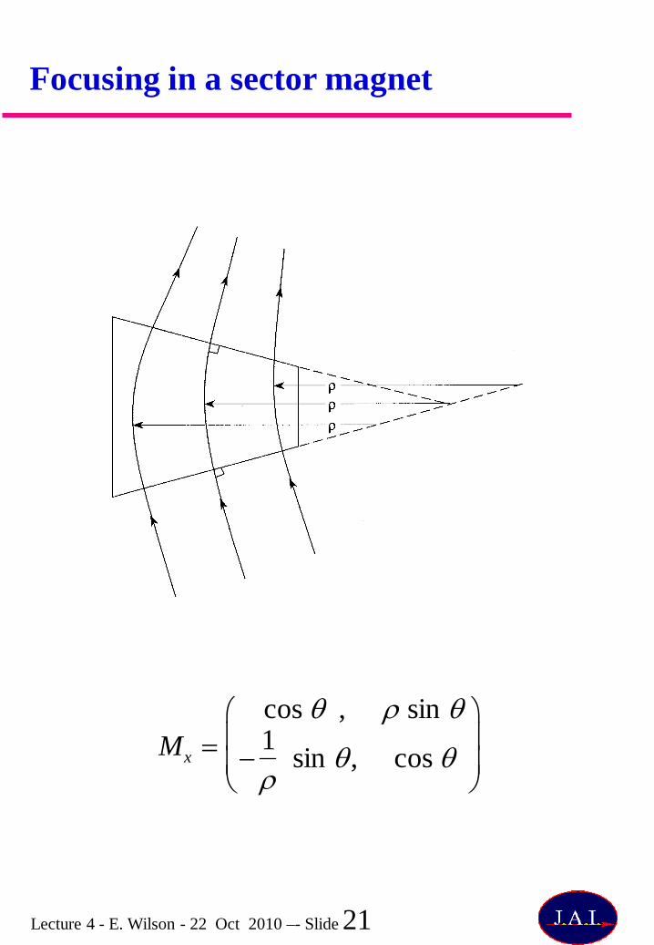
Focusing in a sector magnet

Mx = cos θ , ρ sin θ

−1ρ

sin θ, cos θ


The lattice (1% of SPS)


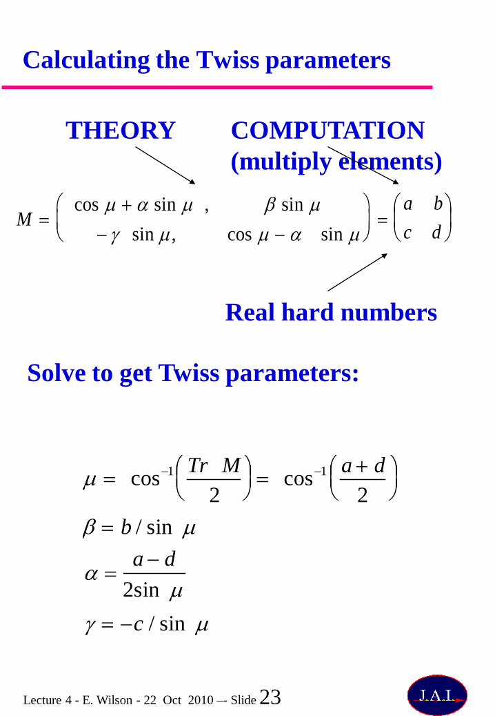
Calculating the Twiss parameters

M =

cos µ + α sin µ , β sin µ− γ sin µ, cos µ − α sin µ

=

a bc d

THEORY COMPUTATION(multiply elements)

Real hard numbers

Solve to get Twiss parameters:

µ = cos−1 Tr M2

= cos−1 a + d

2

β = b / sin µ

α =a − d

2sin µγ = −c / sin µ


Meaning of Twiss parameters

ε is either :» Emittance of a beam anywhere in the ring» Courant and Snyder invariant fro one particle

anywhere in the ring

ε=′β+′α+γ 22 )()(2)( ysyysys


Example of Beam Size Calculation

Emittance at 10 GeV/cε = 20π mm.mrad = 20π ×10−6 m.radˆ β = 108 m

= 46 10−6

= 46.10−3 m= 46 mm.

εβ = 108.20.10−6

= 0.43 10−6

= 0.43.10−3 rad= 0.43 mrad.

εβ = 20.10−6

108

x

′ x



Summary


Check Solution of Hill Twiss Matrix Solving for a ring The lattice Beam sections Physical meaning of Q and beta Smooth approximation

Date post:	31-May-2020
Category:	Documents
Upload:	others
View:	2 times
Download:	0 times

Lecture 4 - Transverse Optics II · Lecture 4 - E. Wilson - 22 Oct 2010 –-Slide2 Contents of...

Documents