BENG 221

Lecture 4Tutorial

Overview

Example: RingOscillatorDynamics

Analytic ODESolution

NumericalVerification

NumericalSimulation

Further Reading

4.1

BENG 221Mathematical Methods in Bioengineering

Lecture 4

TutorialAnalytic and Numerical Methods in ODEs

Gert CauwenberghsDepartment of Bioengineering

UC San Diego

BENG 221

Lecture 4Tutorial

Overview

Example: RingOscillatorDynamics

Analytic ODESolution

NumericalVerification

NumericalSimulation

Further Reading

4.2

Summary

We will review analytic and numerical techniques for solvingODEs, using pencil and paper, and implemented in Matlab.These simple techniques lay the foundations for solving morecomplex systems of PDEs in the coming weeks.

By way of example we study the dynamics of a ring oscillator, acircular chain of three inverters with identical capacitive loading.

BENG 221

Lecture 4Tutorial

Overview

Example: RingOscillatorDynamics

Analytic ODESolution

NumericalVerification

NumericalSimulation

Further Reading

4.3

Today’s Coverage:

Example: Ring Oscillator Dynamics

Analytic ODE Solution

Numerical Verification

Numerical Simulation

BENG 221

Lecture 4Tutorial

Overview

Example: RingOscillatorDynamics

Analytic ODESolution

NumericalVerification

NumericalSimulation

Further Reading

4.4

Some circuit elements

Figure: An invertingtransconductor (inverter)converts and input voltage to anoutput current, with gain −G.

Figure: A capacitor convertscharge, or integrated current, tovoltage with gain 1/C.

iout = g(vin) ≈ −Gvin (1) v =QC

=1C

∫ t

−∞i dt (2)

BENG 221

Lecture 4Tutorial

Overview

Example: RingOscillatorDynamics

Analytic ODESolution

NumericalVerification

NumericalSimulation

Further Reading

4.5

Ring Oscillator

Figure: A 3-inverter ring oscillator with capacitive loading.

Cdv1

dt= g(v3) ≈ −G v3

Cdv2

dt= g(v1) ≈ −G v1 (3)

Cdv3

dt= g(v2) ≈ −G v2

v1(0) = v10

v2(0) = v20 (4)v3(0) = v30

BENG 221

Lecture 4Tutorial

Overview

Example: RingOscillatorDynamics

Analytic ODESolution

NumericalVerification

NumericalSimulation

Further Reading

4.6

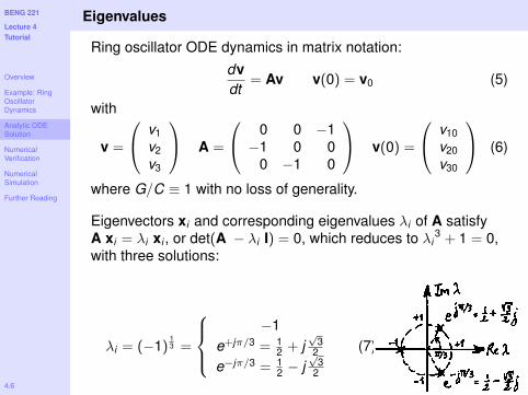
Eigenvalues

Ring oscillator ODE dynamics in matrix notation:dvdt

= Av v(0) = v0 (5)

with

v =

v1v2v3

A =

0 0 −1−1 0 0

0 −1 0

v(0) =

v10v20v30

(6)

where G/C ≡ 1 with no loss of generality.

Eigenvectors xi and corresponding eigenvalues λi of A satisfyA xi = λi xi , or det(A − λi I) = 0, which reduces to λi

3 + 1 = 0,with three solutions:

λi = (−1)13 =

−1

e+jπ/3 = 12 + j

√3

2e−jπ/3 = 1

2 − j√

32

(7)

BENG 221

Lecture 4Tutorial

Overview

Example: RingOscillatorDynamics

Analytic ODESolution

NumericalVerification

NumericalSimulation

Further Reading

4.7

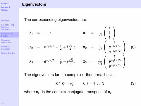
Eigenvectors

The corresponding eigenvectors are:

λ1 = −1 : x1 = 1√3

111

λ2 = e+jπ/3 = 1

2 + j√

32 : x2 = 1√

3

1e+j2π/3

e−j2π/3

λ3 = e−jπ/3 = 1

2 − j√

32 : x3 = 1√

3

1e−j2π/3

e+j2π/3

(8)

The eigenvectors form a complex orthonormal basis:

xi∗ xj = δij , i , j = 1, . . .3 (9)

where xi∗ is the complex conjugate transpose of xi .

BENG 221

Lecture 4Tutorial

Overview

Example: RingOscillatorDynamics

Analytic ODESolution

NumericalVerification

NumericalSimulation

Further Reading

4.8

Eigenmodes

The general solution is the superposition of eigenmodes (seeLecture 1):

v =3∑

i=1

ci xi eλi t

= c1 e−t 1√3

111

+ (10)

c2 e12 t ej

√3

2 t 1√3

1e+j2π/3

e−j2π/3

+

c3 e12 t e−j

√3

2 t 1√3

1e−j2π/3

e+j2π/3

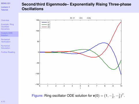
v(t) is real, and so c2 and c3 must be complex conjugate.Therefore, the second and third eigenmodes are oscillatory withan exponentially rising carrier. The first eigenmode is a decayingexponential common-mode transient.

BENG 221

Lecture 4Tutorial

Overview

Example: RingOscillatorDynamics

Analytic ODESolution

NumericalVerification

NumericalSimulation

Further Reading

4.9

First Eigenmode– Common-mode Decaying Exponential

0 1 2 3 4 5 6 7 8 9 100

0.2

0.4

0.6

0.8

1

1.2

t

IC: (1 1 1)

v1v2v3

Figure: Ring oscillator ODE solution for v(0) = (1, 1, 1)T .

BENG 221

Lecture 4Tutorial

Overview

Example: RingOscillatorDynamics

Analytic ODESolution

NumericalVerification

NumericalSimulation

Further Reading

4.10

Second/third Eigenmode– Exponentially Rising Three-phaseOscillations

0 1 2 3 4 5 6 7 8 9 10−150

−100

−50

0

50

100

150

t

IC: (1 −0.5 −0.5)

v1v2v3

Figure: Ring oscillator ODE solution for v(0) = (1,− 12 ,−

12 )

T .

BENG 221

Lecture 4Tutorial

Overview

Example: RingOscillatorDynamics

Analytic ODESolution

NumericalVerification

NumericalSimulation

Further Reading

4.11

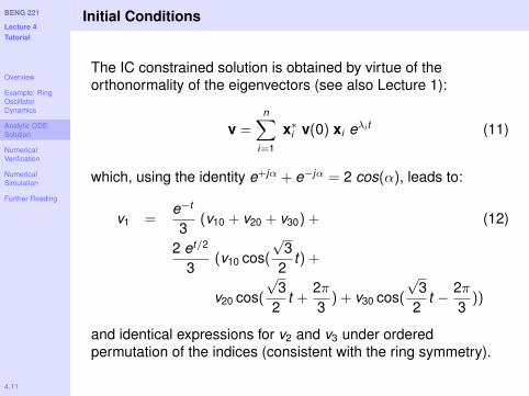
Initial Conditions

The IC constrained solution is obtained by virtue of theorthonormality of the eigenvectors (see also Lecture 1):

v =n∑

i=1

x∗i v(0) xi eλi t (11)

which, using the identity e+jα + e−jα = 2 cos(α), leads to:

v1 =e−t

3(v10 + v20 + v30) + (12)

2 et/2

3(v10 cos(

√3

2t) +

v20 cos(

√3

2t +

2π3

) + v30 cos(

√3

2t − 2π

3))

and identical expressions for v2 and v3 under orderedpermutation of the indices (consistent with the ring symmetry).

BENG 221

Lecture 4Tutorial

Overview

Example: RingOscillatorDynamics

Analytic ODESolution

NumericalVerification

NumericalSimulation

Further Reading

4.12

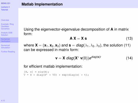
Matlab Implementation

Using the eigenvector-eigenvalue decomposition of A in matrixform:

A X = X s (13)

where X = (x1,x2,x3) and s = diag(λ1, λ2, λ3), the solution (11)can be expressed in matrix form:

v = X diag(X∗ v(0))ediag(s)t (14)

for efficient matlab implementation:[X, s] = eig(A);V = X * diag(X’ * V0) * exp(diag(s) * t);

BENG 221

Lecture 4Tutorial

Overview

Example: RingOscillatorDynamics

Analytic ODESolution

NumericalVerification

NumericalSimulation

Further Reading

4.13

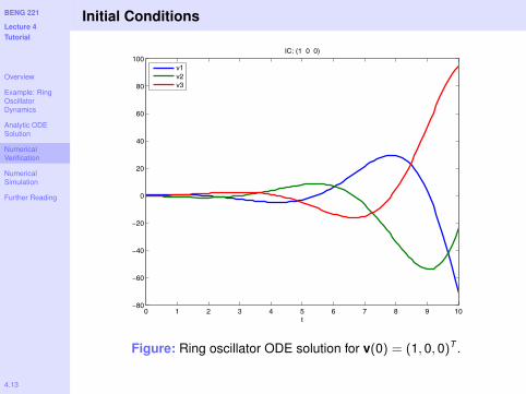
Initial Conditions

0 1 2 3 4 5 6 7 8 9 10−80

−60

−40

−20

0

20

40

60

80

100

t

IC: (1 0 0)

v1v2v3

Figure: Ring oscillator ODE solution for v(0) = (1, 0, 0)T .

BENG 221

Lecture 4Tutorial

Overview

Example: RingOscillatorDynamics

Analytic ODESolution

NumericalVerification

NumericalSimulation

Further Reading

4.14

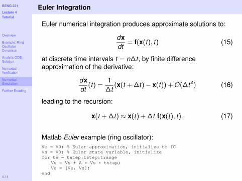
Euler Integration

Euler numerical integration produces approximate solutions to:

dxdt

= f(x(t), t) (15)

at discrete time intervals t = n∆t , by finite differenceapproximation of the derivative:

dxdt

(t) =1

∆t(x(t + ∆t)− x(t)) +O(∆t2) (16)

leading to the recursion:

x(t + ∆t) ≈ x(t) + ∆t f(x(t), t). (17)

Matlab Euler example (ring oscillator):Ve = V0; % Euler approximation, initialize to ICVs = V0; % Euler state variable, initializefor te = tstep:tstep:trange

Vs = Vs + A * Vs * tstep;Ve = [Ve, Vs];

end

BENG 221

Lecture 4Tutorial

Overview

Example: RingOscillatorDynamics

Analytic ODESolution

NumericalVerification

NumericalSimulation

Further Reading

4.15

Euler Integration

0 1 2 3 4 5 6 7 8 9 10−100

−50

0

50

100

150

t

IC: (1 0 0)

v1v2v3

Figure: Ring oscillator ODE simulation using Euler integration.

BENG 221

Lecture 4Tutorial

Overview

Example: RingOscillatorDynamics

Analytic ODESolution

NumericalVerification

NumericalSimulation

Further Reading

4.16

Crank-Nicolson Integration

Better numerical ODE methods exist that use higher-order finitedifference approximations of the derivative. Crank-Nicolson is asecond order method that approximates (15) more accuratelyusing a centered version of the finite difference approximation ofthe derivative:

dxdt

(t +∆t2

) =1

∆t(x(t + ∆t)− x(t)) +O(∆t3) (18)

leading to a recursion:

x(t + ∆t) ≈ x(t) + ∆t f(x(t +∆t2

), t +∆t2

)

≈ x(t) +∆t2

(f(x(t), t) + f(x(t + ∆t), t + ∆t)).(19)

Matlab CN example (ring oscillator):G = (eye(3) - A * tstep / 2) \ (eye(3) + A * tstep / 2);Vc = V0; % CN approximation, initialize to ICVs = V0; % CN state variable, initializefor te = tstep:tstep:trange

Vs = G * Vs;Vc = [Vc, Vs];

end

BENG 221

Lecture 4Tutorial

Overview

Example: RingOscillatorDynamics

Analytic ODESolution

NumericalVerification

NumericalSimulation

Further Reading

4.17

Crank-Nicolson Integration

0 1 2 3 4 5 6 7 8 9 10−80

−60

−40

−20

0

20

40

60

80

100

t

IC: (1 0 0)

v1v2v3

Figure: Ring oscillator ODE simulation using Crank-Nicolsonintegration.

BENG 221

Lecture 4Tutorial

Overview

Example: RingOscillatorDynamics

Analytic ODESolution

NumericalVerification

NumericalSimulation

Further Reading

4.18

Higher-Order Integration

Crank-Nicolson (19) is implicit in that the solution at time stept + ∆t is recursive in the state variable x(t + ∆t), rather thanforward e.g., given in previous values of the state variable x(t).More advanced methods, such as Runge-Kutta and several ofMatlab’s built-in ODE solvers, are explicit and/or higher order,allowing faster integration although possibly at the expense ofnumerical stability.

Matlab ode23 example (ring oscillator):OdeOptions = odeset(’RelTol’, 1e-9); % accuracy, pleasedVdt = @(t,V) A * V;[tm, Vm] = ode23(dVdt, [0 trange], V0);

BENG 221

Lecture 4Tutorial

Overview

Example: RingOscillatorDynamics

Analytic ODESolution

NumericalVerification

NumericalSimulation

Further Reading

4.19

Explicit Forward Second-Order Integration

0 1 2 3 4 5 6 7 8 9 10−80

−60

−40

−20

0

20

40

60

80

100

t

IC: (1 0 0)

v1v2v3

Figure: Ring oscillator ODE simulation using an explicit version ofCrank-Nicolson integration using a forward series expansion up tosecond order.

BENG 221

Lecture 4Tutorial

Overview

Example: RingOscillatorDynamics

Analytic ODESolution

NumericalVerification

NumericalSimulation

Further Reading

4.20

Matlab Built-in ode23 Solver

0 1 2 3 4 5 6 7 8 9 10−80

−60

−40

−20

0

20

40

60

80

100

t

IC: (1 0 0)

v1v2v3

Figure: Ring oscillator ODE simulation using the Matlab built-in ode23numeric ODE solver.

BENG 221

Lecture 4Tutorial

Overview

Example: RingOscillatorDynamics

Analytic ODESolution

NumericalVerification

NumericalSimulation

Further Reading

4.21

Bibliography

R. Haberman, Applied Partial Differential Equations withFourier Series and Boundary Value Problems, 4th Ed., 2004,Ch. 6.

Wikipedia, Conjugate Transpose, http://en.wikipedia.org/wiki/Conjugate_transpose.

Wikipedia, Numerical Ordinary Differential Equations,http://en.wikipedia.org/wiki/Numerical_ordinary_differential_equations.

Wikipedia, Runge Kutta Methods, http://en.wikipedia.org/wiki/Runge-Kutta_methods.