Lecture 5

Optimal portfolios

Learning outcomes

• By the end of this lecture you should: – Be familiar with the separation theorem

– Know why this implies that every investor’s optimal risky portfolio is the market portfolio

– Be able to solve the portfolio problem in the presence of a risk free asset and the market portfolio

– Understand how this implies the CAPM

The optimal portfolio

• Last time we found the optimal portfolio by picking the portfolio on the efficient frontier that touched our highest indifference curve (gave the highest utility).

E(r)

σ

Introduce a risk free asset

• Suppose that in addition to the risky assets that we talked about last lecture, we could also invest in some risk free asset

• We’ll call the return of this asset the risk free return, rf

• By definition of risk free, we have • During our first three lecture we were only

concerned with these kind of assets • For simplicity we will assume that we have a flat

and constant term structure of interest rates

( ) ff rrE =( ) 0=frVar

Combining the risk free asset with a risky portfolio into a complete portfolio

• Suppose we want to combine some risky portfolio, P, with the risk free asset

• Let’s denote the fraction invested in the risky asset y and the fraction invested in the risk free asset (1-y)

• The return of our complete portfolio, C, is defined as before:

( ) PfC yrryr +−= 1

The expected return of a complete portfolio

• As usual, we are interested in the risk and expected return of this portfolio. Lets start with the expected return:

• Like before the portfolio expected return is a weighted average of the asset expected returns

• It will be convenient to express this equation as:

• By varying y, we can choose our expected return

( ) ( )[ ]( ) ( ) ( )PfC

PfC

ryEryrEyrryErE

+−=

+−=

1

1

( ) ( )[ ]fPfC rrEyrrE −+=

The risk of a complete portfolio

• We figured out in the last lecture how to calculate the variance of a two asset portfolio:

• The neat thing here is that rf is a constant, so Var(rf) = 0 and Cov(rf, rP) = 0:

• We find that σC is linear in σP

( )( ) ( )[ ]( ) ( ) ( ) ( ) ( ) ( )PfPfC

PfC

PfC

rryCovyrVaryrVaryrVar

yrryVarrVaryrryr

,121

1

1

22 −++−=

+−=

+−=

( ) ( )

PPC

PPC

yy

yrVaryrVar

σσσ

σ

==

==22

222

These are linear combinations

• We have found that:

• So y determines what fraction of the distance between the risk free asset and P is covered in both dimensions

• When y = 0 we are in the risk free asset, e.g. σC = 0 and E(RC) = rf

• When y = 0.5 we are halfway between the risk free asset and P, e.g. σC = 0.5σP and E(RC) = rf + 0.5[E(RC) - rf]

• When y = 1 we are in portfolio P, e.g. σC = σP and E(RC) = E(RP)

( ) ( )[ ]PC

fPfC

yrrEyrrE

σσ =

−+=

Let’s plot it

• Graphically, this means that all our complete portfolios plot on a straight line between the risk free asset and P

• Let’s call the line associated with the risky portfolio P for CALP (for reasons that will become clear later)

E(r)

σ

rf

P CALP

Let’s plot it

• Last lecture, we learned only to consider risky portfolios on the efficient frontier, so let’s chose P from that set

E(r)

σ

rf

P CALP

Apply the mean variance criterion

• We see that some of our complete portfolios dominate some portfolios on the efficient frontier

• Which ones are dominated depends on the risky portfolio we choose

E(r)

σ

rf

P1

P2

CALP1

CALP2

Apply the mean variance criterion

• We’re interested in choosing the P that dominates the most portfolios

• This turns out to be the portfolio where the line of complete portfolios is tangent to the efficient frontier

• We call this P the optimal risky portfolio, P*

• The associated line CALP* is often simply denoted CAL

E(r)

σ

rf

P*

CALP* = CAL

Apply the mean variance criterion

• A different way to phrase this is to note that we only consider risky portfolios on the efficient frontier

• We can then forget about the efficient frontier and only compare CALs

• We note that for any portfolio on CAL1 there is a dominating portfolio just above it on CAL2

• Portfolios on CALs with higher slopes will always dominate portfolios on CALs with lower slopes

• The optimal risky portfolio is the portfolio associated with the CAL that has the highest slope

E(r)

σ

rf

CAL1

CAL2

The optimal risky portfolio

• All portfolios other than P* on the efficient frontier are dominated by some combination of the optimal risky portfolio, P*, and the risk free asset

• This means that all efficient portfolios consist of some such combination

• The reason we call the corresponding line CAL is that all capital will be allocated along it

• CAL is an acronym for the Capital Allocation Line

The separation theorem

• All efficient portfolios (in the presence of a risk free asset) are on the CAL

• The CAL is determined by the optimal risky portfolio • We pick the portfolio on the CAL that offers the

amount of risk we want to take. This is expressed in our choice of y.

• Thus, our entire portfolio choice problem can be separated into two parts: – Find the optimal risky portfolio, P*

– Choose how much risk we want by choosing the fraction of our wealth that we invest in that portfolio, y

Step 1: Choosing P* (and implicitly the CAL)

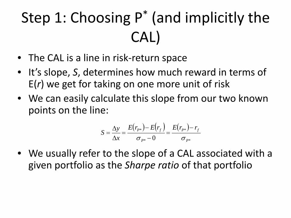
• The CAL is a line in risk-return space • It’s slope, S, determines how much reward in terms of

E(r) we get for taking on one more unit of risk • We can easily calculate this slope from our two known

points on the line:

• We usually refer to the slope of a CAL associated with a given portfolio as the Sharpe ratio of that portfolio

( ) ( ) ( )*

*

*

*

0 P

fP

P

fP rrErErExyS

σσ−

=−

−=

∆∆

=

Step 1: Choosing P*

• Recall from the construction of our utility function that we only care about E(r) and σ

• This means we always prefer a higher Sharpe ratio, S • We find the optimal portfolio, P*, by choosing its

portfolio weights, wP, so as to maximizes SP:

• This gets messy (at least when we can choose between many assets)

• You can do this using the Excel solver or some other suitable computer program

( )P

fPPw

rrES

P σ−

=max

Step 2: Choosing the risky share, y

• We choose y according to our risk preference, which is modeled in our utility function by A

• We may again illustrate this choice using indifference curves:

E(r)

σ

rf

P*

C

Step 2: Choosing the risky share, y

• Once we have determined P*, we know from before that our risk and return will be:

• We also know that our utility will depend on these quantities in the following manner:

• Let’s combine these equations:

( )[ ] ( ) ( )[ ] 2*

22

1*

2*2

1* PfPfPfPf AyrrEyryArrEyrU σσ −−+=−−+=

( ) 22

1 σArEU −=

( ) ( )[ ]PC

fPfC

yrrEyrrE

σσ =

−+=

Step 2: Choosing the risky share, y

• By choosing y, we choose where to end up on the CAL • Let’s choose y so as to maximize our utility: • We set the first derivative equal to zero and solve for y:

• is known as the reward-to-risk ratio (and has an interpretation that is very similar to the Sharpe ratio)

• y* is increasing in this ratio, meaning that the more rewards in terms of E(r) we get for taking on extra risk, the more we invest in the risky portfolio

• y* is decreasing in A, meaning that the more risk-averse we are, the less we invest in the risky portfolio

( )[ ] 2*

22

1*max PfPfy

AyrrEyrU σ−−+=

( )[ ]( ) ( )

2*

*2

*

**

2**

1

0

P

fP

P

fP

PfP

rrEAA

rrEy

AyrrEyU

σσ

σ

−⋅=

−=

=−−=∂∂

( )2

*

*

P

fP rrEσ

−

Leveraged positions

• There is nothing in principle that prevents us from choosing y > 1

• This means that we’ll take a short position in the risk-free asset, i.e. (1 - y) < 0

• The interpretation of this is that we borrow money

• We say that we take a leveraged position in P*

Borrowing constraints

• In practice, we must borrow at a higher rate than we can invest at

• This is because lending money to us is not really risk free

• Graphically we get a kink in the CAL when y = 1

• Since we’d have higher default risks for more leveraged positions, the CAL may also be concave when y > 1

Implications of the separation theorem

• The rational way to increase risk taking is to increase leverage (not to buy more tech stocks)

• All investors will end up holding the same risky portfolio

• Since prices adjust to set the supply of stocks equal to the demand for stocks, the portfolio demanded must be the portfolio supplied

• P* is the market portfolio, M

Implications of the separation theorem

• The attractiveness of a stock is determined by its risk and return effects on this portfolio

• We saw last lecture that the expected return effect of a stock on a portfolio is linear and that the risk effect depends crucially on its covariance with the other stocks in the portfolio

A note on expected returns • A company that issues a stock is basically selling a claim to its future

profits • These profits are determined by the operations of the company • Since the profits are risky, the company has to sell the claims at a price

that is lower than their expected value • If the price is lower, the expected return of the investors is higher • Since these high expected returns are used to induce investors to hold

“unattractive” risky stocks, high expected returns signify “unattractive” stocks, which may seem counterintuitive

• Of course, high expected returns are not themselves unattractive • In equilibrium, expected returns are set so as to make all stocks equally

attractive • Some times we emphasize this by referring to a stocks expected return as

its required return (to make it as attractive as all other stocks)

The market portfolio

• Recall that the market portfolio is the optimal risky portfolio for all investors

• Each investor buys a small fraction of the portfolio

• The entire market portfolio simply consists of all assets

• Just like in other portfolios, the weight of each asset in the market portfolio is the assets total market value divided by the total value of the portfolio:

∑=

jj

ii V

Vw

The expected return of the market portfolio

• The return of the market portfolio, rM, is

• We calculate expectations just like with any other portfolio

• It is clear that the contribution of asset i to the expected return of the

market portfolio is

• It will be useful to express this as the contribution of asset i to the market portfolios excess return, i.e. its return over and above the risk-free rate

• The contribution of asset i to the market excess return is

∑=

=N

iiiM rwr

1

( ) ( )[ ]∑=

−=−N

ifiifM rrEwrrE

1

( )ii rEw

( ) ( )∑=

=N

iiiM rEwrE

1

( )[ ]fii rrEw −

The variance of the market portfolio

• We calculate the variance just like any other portfolio variance, i.e. by setting up the covariance matrix and summing the elements:

• Note that every asset corresponds to one row in the matrix

w1r1 w2r2 … wNrN

w1r1 Cov(w1r1,w1r1) Cov(w1r1,w2r2) … Cov(w1r1,wNrN)

w2r2 Cov(w2r2,w1r1) Cov(w2r2,w2r2) … Cov(w2r2,wNrN)

… … … …

wNrN Cov(wNrN,w1r1) Cov(wNrN,w2r2) … Cov(wNrN,wNrN)

The variance of the market portfolio

• The contribution of each asset to the variance of the market portfolio is captured by the sum of the elements in its row

• Let’s view the row for asset i in isolation:

• This matrix corresponds to the matrix we would set up to calculate

w1r1 w2r2 … wNrN

wiri Cov(w1r1,w1r1) Cov(w1r1,w2r2) … Cov(w1r1,wNrN)

∑=

N

jjjii rwrwCov

1,

The risk-return ratio of the market portfolio

• We see that the contribution of asset i to the variance of the market portfolio is

• Note that the reward-to-risk ratio of the market portfolio is:

• The contribution of asset i to this ratio is:

( ) ( )MiiMii

N

jjjii rrCovwrrwCovrwrwCov ,,,

1==

∑=

( )2M

fM rrEσ

−

( )[ ]( )

( )( )Mi

fi

Mii

fii

rrCovrrE

rrCovwrrEw

,,−

=−

The risk-return ratio of the market portfolio

• Since the market portfolio is the portfolio with the best risk-return ratio, it cannot be improved by changing the portfolio weights

• This means that no isolated investment can make a larger contribution to the risk-return ratio than any other investment:

• This is also true for the market portfolio itself:

( )( )

( )( )Mj

fj

Mi

fi

rrCovrrE

rrCovrrE

,,−

=−

( )( )

( )( )

( )2,, M

fM

MM

fM

Mi

fi rrErrCovrrE

rrCovrrE

σ−

=−

=−

The CAPM

• We can rewrite this equation as

• This equation expresses a relation that must hold between an asset’s expected return and its covariance with the market

• We call this model the Capital Asset Pricing Model or the CAPM

• It will be the focus of our coming lectures

( )( )

( )

( ) ( ) ( )

2

2

,

,

i f M f

i M M

i Mi f M f

M

E r r E r rCov r r

Cov r rE r r E r r

σ

σ

− −=

= + −