2/11/2016

1

ECE 5322 21st Century Electromagnetics

Instructor:Office:Phone:E‐Mail:

Dr. Raymond C. RumpfA‐337(915) 747‐6958rcrumpf@utep.edu

Coupled-Mode Theory

Lecture #5

Lecture 5 1

Lecture Outline

• Electromagnetic modes

• Coupled-mode theory

• Codirectional coupling

• Contradirectional coupling

• Non-directional coupling

• Phase matching with gratings

• Mode-matching vs. coupled-wave models

Lecture 5 Slide 2

2/11/2016

2

Electromagnetic Modes

What are modes?

Lecture 5 Slide 4

Modes can mean many different things depending on the context it is being used.

• Different discrete eigen‐modes in a waveguide• Different polarizations• Different directions• Etc.

Generalized Definition:

An electromagnetic mode is electromagnetic power that exists independent and different from other electromagnetic power.

2/11/2016

3

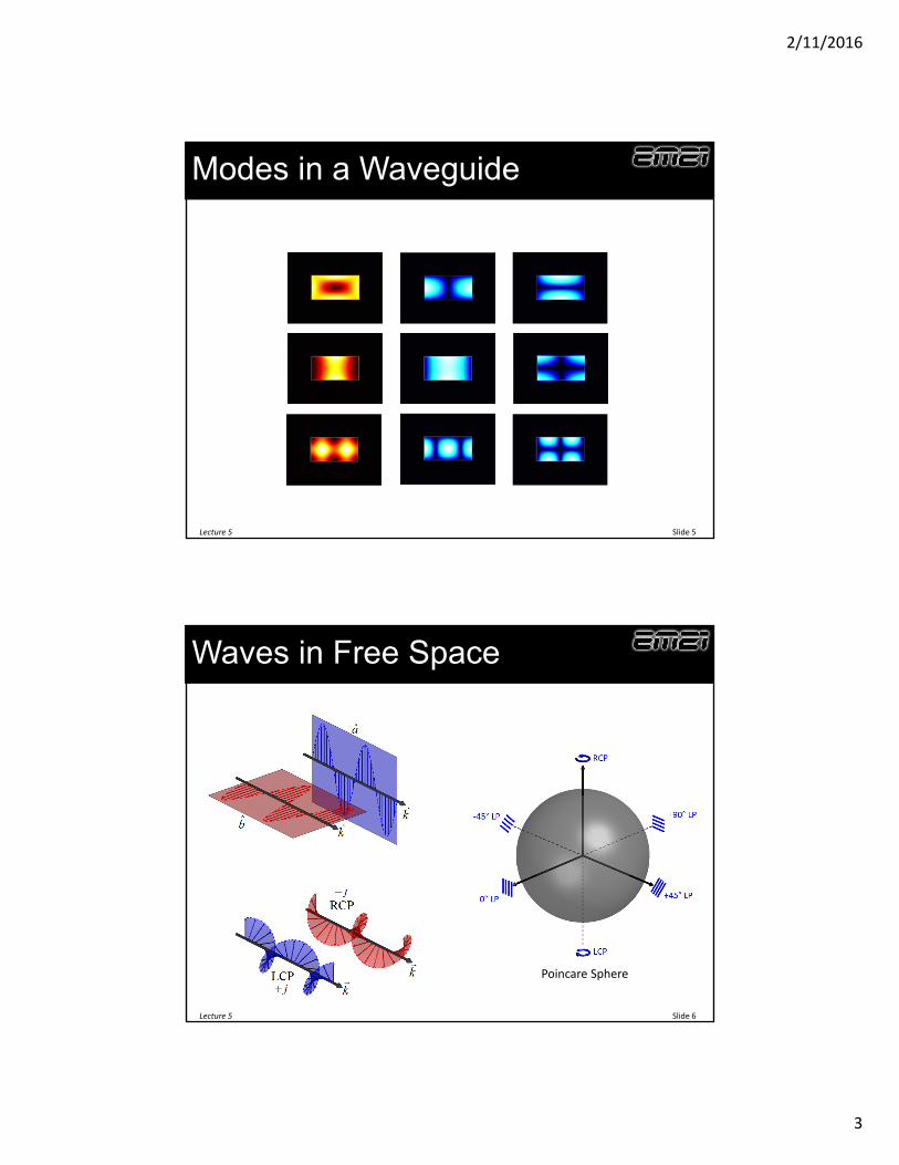
Modes in a Waveguide

Lecture 5 Slide 5

Waves in Free Space

Lecture 5 Slide 6

Poincare Sphere

2/11/2016

4

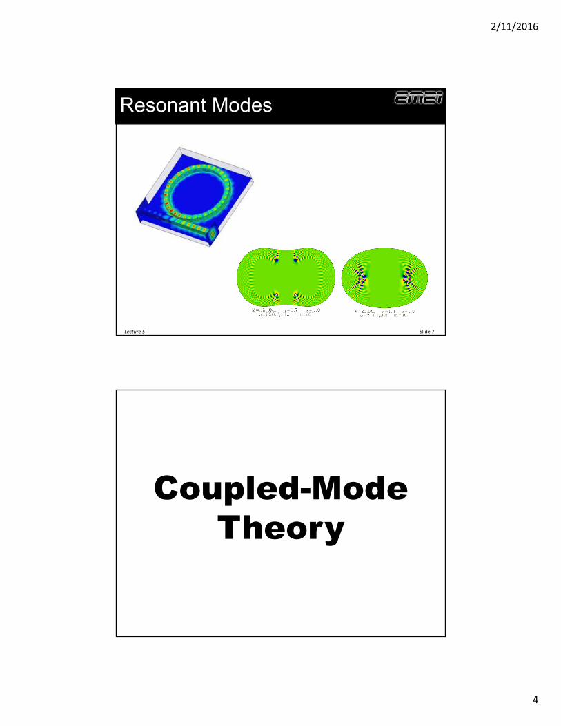
Resonant Modes

Lecture 5 Slide 7

Coupled-Mode Theory

2/11/2016

5

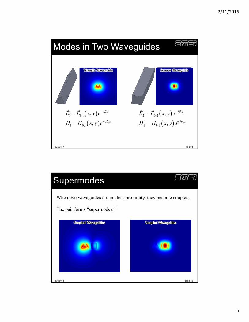
Modes in Two Waveguides

Lecture 5 Slide 9

Triangle Waveguide Square Waveguide

1

1

1 0,1

1 0,1

,

,

j z

j z

E E x y e

H H x y e

2

2

2 0,2

2 0,2

,

,

j z

j z

E E x y e

H H x y e

Supermodes

Lecture 5 Slide 10

Coupled WaveguidesCoupled Waveguides

When two waveguides are in close proximity, they become coupled.

The pair forms “supermodes.”

2/11/2016

6

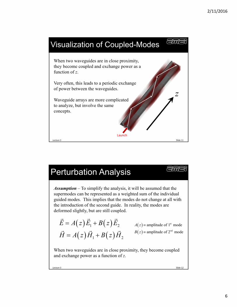
Visualization of Coupled-Modes

Lecture 5 Slide 11

When two waveguides are in close proximity, they become coupled and exchange power as a function of z.

Very often, this leads to a periodic exchange of power between the waveguides.

Waveguide arrays are more complicatedto analyze, but involve the same concepts.

z

Launch

Perturbation Analysis

Lecture 5 Slide 12

1 2

1 2

E A z E B z E

H A z H B z H

Assumption – To simplify the analysis, it will be assumed that the supermodes can be represented as a weighted sum of the individual guided modes. This implies that the modes do not change at all with the introduction of the second guide. In reality, the modes are deformed slightly, but are still coupled.

When two waveguides are in close proximity, they become coupled and exchange power as a function of z.

st

nd

amplitude of 1 mode

amplitude of 2 mode

A z

B z

2/11/2016

7

Assumed Solution in Perturbation Analysis

Lecture 5 Slide 13

1 2

1 2

E A z E B z E

H A z H B z H

We start with the following solution.

We substitute these into Maxwell’s curl equations to obtain

1 2

1 0 1 1 2 0 2 2

ˆ ˆ 0

ˆ ˆ 0r r

dA dBz E z E

dz dzdA dB

z H j AE z H j BEdz dz

To do this, we made use of the following vector identity

ˆdA

AE A E A E A E z Edz

0

0 r

E j H

H j E

Ignoring magnetic response

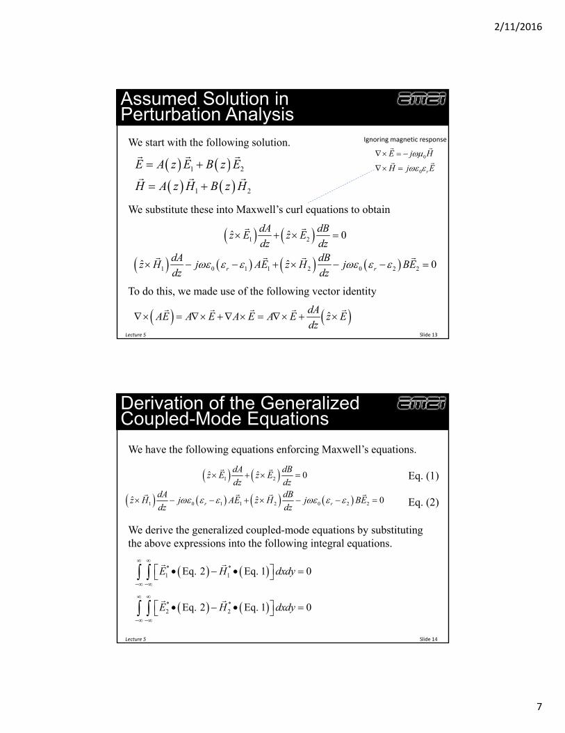
Derivation of the Generalized Coupled-Mode Equations

Lecture 5 Slide 14

We have the following equations enforcing Maxwell’s equations.

We derive the generalized coupled-mode equations by substituting the above expressions into the following integral equations.

1 2

1 0 1 1 2 0 2 2

ˆ ˆ 0

ˆ ˆ 0r r

dA dBz E z E

dz dzdA dB

z H j AE z H j BEdz dz

Eq. (1)

Eq. (2)

* *1 1Eq. 2 Eq. 1 0E H dxdy

* *2 2Eq. 2 Eq. 1 0E H dxdy

2/11/2016

8

Generalized Coupled-Mode Equations

Lecture 5 Slide 15

2 1 2 1

2 1 2 1

12 1 12

21 2 21

0

0

j z j z

j z j z

dA dBc e j A j Be

dz dzdB dA

c e j B j Aedz dz

After LOTS of algebra, we get (i.e. it is easily shown that… )

These are called the generalized coupled-mode equations. These are solved to describe the coupling between the two waveguides.

*0 ,

* *ˆ

r r q p q

pq

p p p p

E E dxdy

z E H E H dxdy

* *

* *

ˆ

ˆ

p p

pq

p p

q

p

q

p

z E H E H dxdy

c

z E H E H dxdy

*0 ,

* *ˆ

r r q p p

p

p p p p

E E dxdy

z E H E H dxdy

Mode Coupling Coefficient Butt Coupling Coefficient Change in Propagation Constant

, 1 or 2p q

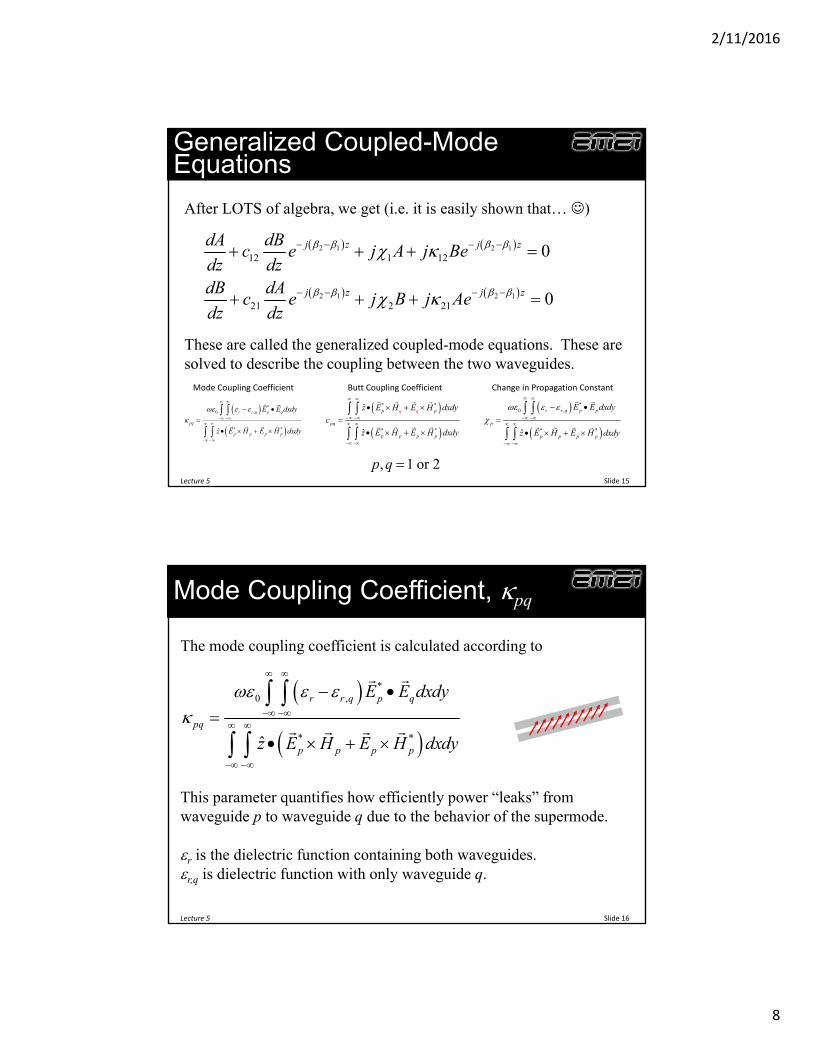
Mode Coupling Coefficient, pq

Lecture 5 Slide 16

*0 ,

* *ˆ

r r q p q

pq

p p p p

E E dxdy

z E H E H dxdy

The mode coupling coefficient is calculated according to

This parameter quantifies how efficiently power “leaks” from waveguide p to waveguide q due to the behavior of the supermode.

r is the dielectric function containing both waveguides. r,q is dielectric function with only waveguide q.

2/11/2016

9

Butt Coupling Coefficient, cpq

Lecture 5 Slide 17

* *

* *

ˆ

ˆ

p p

pq

p p

q

p

q

p

z E H E H dxdy

c

z E H E H dxdy

The coefficient cpq quantifies the excitation efficiency from one waveguide to the other. It is called the butt coupling coefficient and is calculated according to

Butt coupling

Change in Propagation Constant, p

Lecture 5 Slide 18

When the qth waveguide is brought into proximity to pth waveguide, the propagation constant in the pth waveguide changes by p.

*0 ,

* *ˆ

r r q p p

p

p p p p

E E dxdy

z E H E H dxdy

We expect p to be largest when the waveguides are the closest and the fields are perturbed more strongly affecting the propagation constant.

Many analyses just assume = 0.

2/11/2016

10

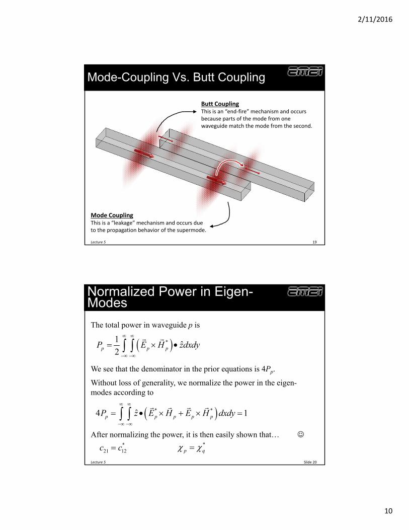
Mode-Coupling Vs. Butt Coupling

Lecture 5 19

Butt CouplingThis is an “end‐fire” mechanism and occurs because parts of the mode from one waveguide match the mode from the second.

Mode CouplingThis is a “leakage” mechanism and occurs due to the propagation behavior of the supermode.

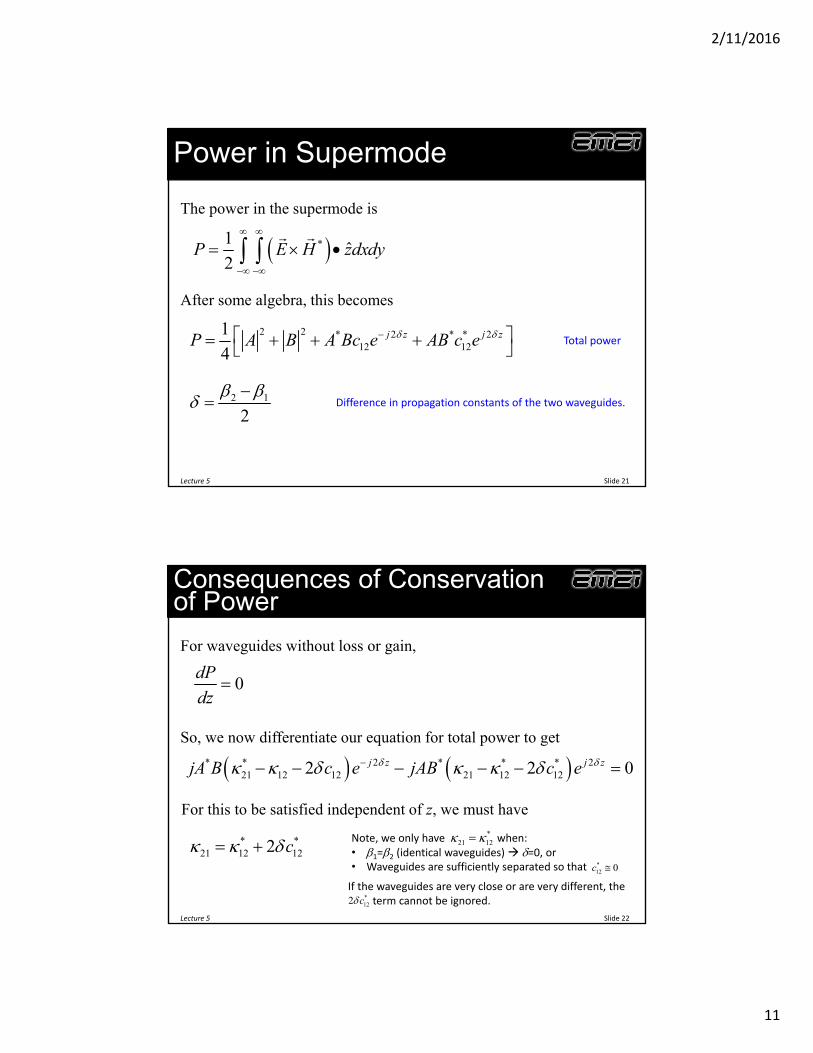
Normalized Power in Eigen-Modes

Lecture 5 Slide 20

The total power in waveguide p is

*1ˆ

2p p pP E H zdxdy

We see that the denominator in the prior equations is 4Pp.

Without loss of generality, we normalize the power in the eigen-modes according to

* *ˆ4 1p p p p pP z E H E H dxdy

After normalizing the power, it is then easily shown that… *

21 12c c *p q

2/11/2016

11

Power in Supermode

Lecture 5 Slide 21

The power in the supermode is

*1ˆ

2P E H zdxdy

After some algebra, this becomes

2 2 * 2 * * 212 12

1

4j z j zP A B A Bc e AB c e

2 1

2

Total power

Difference in propagation constants of the two waveguides.

Consequences of Conservation of Power

Lecture 5 Slide 22

For waveguides without loss or gain,

0dP

dz

So, we now differentiate our equation for total power to get

* * 2 * * * 221 12 12 21 12 122 2 0j z j zjA B c e jAB c e

For this to be satisfied independent of z, we must have

* *21 12 122 c Note, we only have                   when:

• 1=2 (identical waveguides)  =0, or• Waveguides are sufficiently separated so that 

*21 12

*12 0c

If the waveguides are very close or are very different, the term cannot be ignored.*

122 c

2/11/2016

12

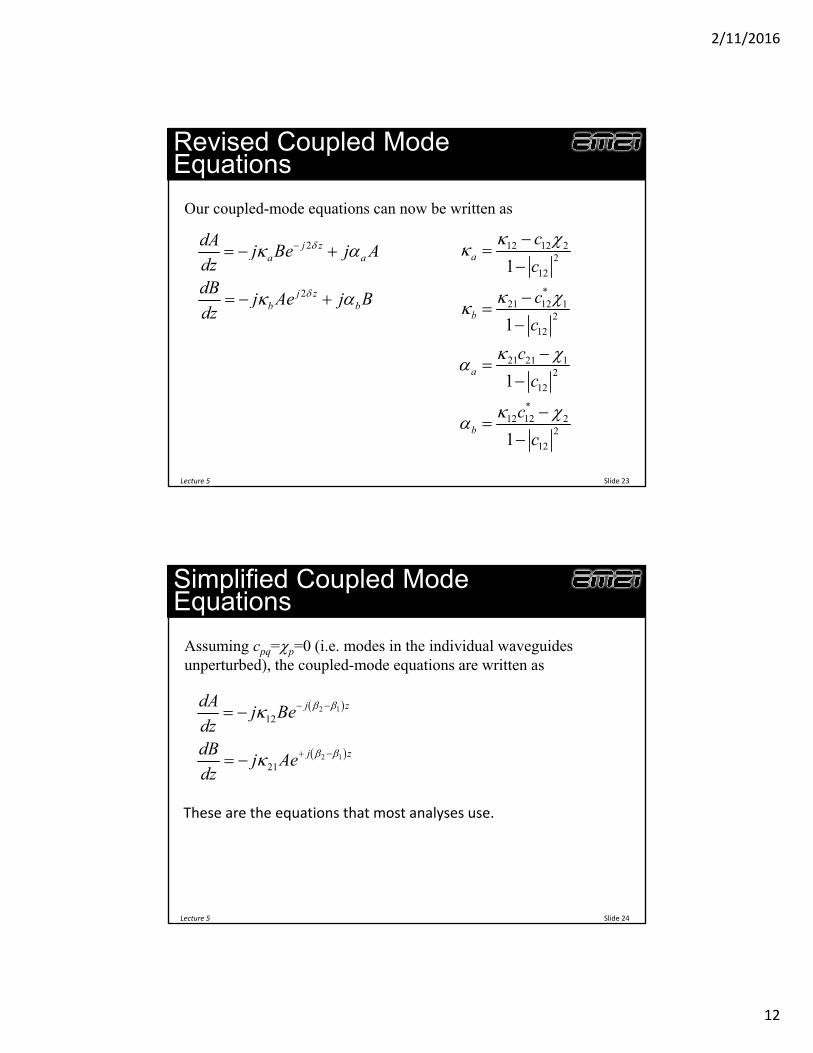
Revised Coupled Mode Equations

Lecture 5 Slide 23

2

2

j za a

j zb b

dAj Be j A

dzdB

j Ae j Bdz

Our coupled-mode equations can now be written as

12 12 22

12

*21 12 1

2

12

21 21 12

12

*12 12 2

2

12

1

1

1

1

a

b

a

b

c

c

c

c

c

c

c

c

Simplified Coupled Mode Equations

Lecture 5 Slide 24

2 1

2 1

12

21

j z

j z

dAj Be

dzdB

j Aedz

Assuming cpq=p=0 (i.e. modes in the individual waveguides unperturbed), the coupled-mode equations are written as

These are the equations that most analyses use.

2/11/2016

13

CodirectionalCoupling

Picture of Codirectional Coupling

Lecture 5 Slide 26

Launch

Exit

2/11/2016

14

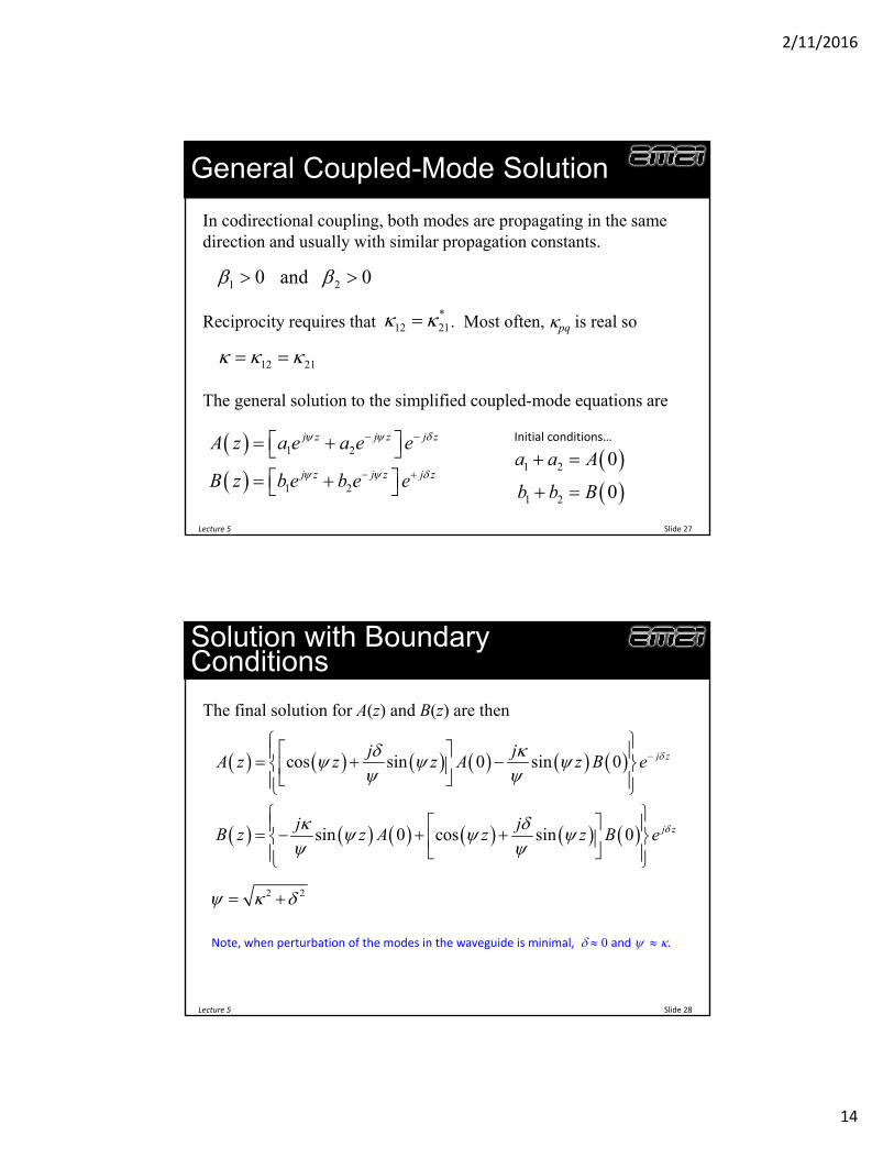
General Coupled-Mode Solution

Lecture 5 Slide 27

1 2

1 2

j z j z j z

j z j z j z

A z a e a e e

B z b e b e e

In codirectional coupling, both modes are propagating in the same direction and usually with similar propagation constants.

The general solution to the simplified coupled-mode equations are

1 20 and 0

Reciprocity requires that . Most often, pq is real so*

12 21

12 21

1 2

1 2

0

0

a a A

b b B

Initial conditions…

Solution with Boundary Conditions

Lecture 5 Slide 28

cos sin 0 sin 0

sin 0 cos sin 0

j z

j z

j jA z z z A z B e

j jB z z A z z B e

The final solution for A(z) and B(z) are then

2 2

Note, when perturbation of the modes in the waveguide is minimal,  0 and  .

2/11/2016

15

Typical Solution in Terms of Power

Lecture 5 Slide 29

0 0cos sin sinj z j zj jA z A z z e B z A z e

In most cases, power is injected into only one waveguide.

00 0 0A A B

Our equations for A(z) and B(z) reduce to

It is often more meaningful to write similar expressions in terms of the power in each waveguide as a function of z.

2

22

0

2

22

0

1 sin

sin

a

b

A zP z F z

A

B zP z F z

A

2

2

1

1F

Maximum power‐coupling efficiency…

Typical Response of Codirectional Couplers

Lecture 5 Slide 30

2 3 2 2

2 3 2 2

0 1F

2 0.2F

Maximums occur at

2 1 0,1,2,...2mz m m

Coupling LengthThe length over which maximum power is transferred to the second waveguide is called the coupling length.

When 1=2 (i.e.  = 0),

2 22 2cL

2cL

2/11/2016

16

Visualization of the Terms

Lecture 5 Slide 31

z

Launch

cL

sin

sin2

cL

2

4

2

c

c

L

L

ContradirectionalCoupling

(Bragg Grating)

2/11/2016

17

Contradirectional Coupling

Lecture 5 Slide 33

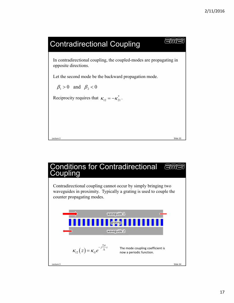
In contradirectional coupling, the coupled-modes are propagating in opposite directions.

Let the second mode be the backward propagation mode.

1 20 and 0

Reciprocity requires that .*12 21

Conditions for ContradirectionalCoupling

Lecture 5 Slide 34

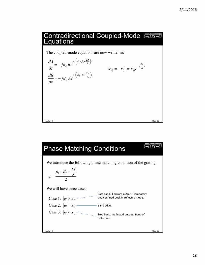
Contradirectional coupling cannot occur by simply bringing two waveguides in proximity. Typically a grating is used to couple the counter propagating modes.

waveguide 1

waveguide 2

grating

2

12

j z

Gz e

The mode coupling coefficient is now a periodic function.

2/11/2016

18

Contradirectional Coupled-Mode Equations

Lecture 5 Slide 35

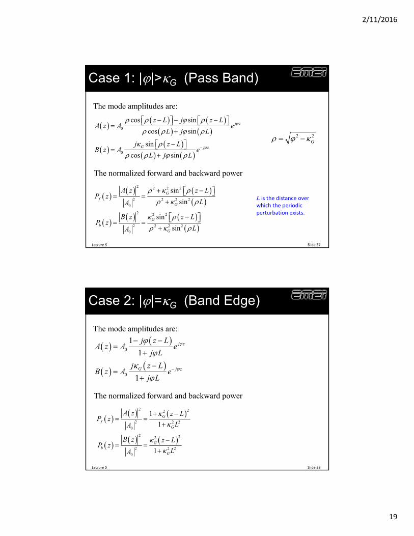
The coupled-mode equations are now written as

2 1

2 1

2

2

j z

G

j z

G

dAj Be

dz

dBj Ae

dz

2*

12 21

j z

Ge

Phase Matching Conditions

Lecture 5 Slide 36

1 2

2

2

We introduce the following phase matching condition of the grating.

We will have three cases

Case 1:

Case 2:

Case 3:

G

G

G

Band edge.

Pass band.  Forward output.  Temporary and confined peak in reflected mode.

Stop band.  Reflected output.  Band of reflection.

2/11/2016

19

Case 1: ||>G (Pass Band)

Lecture 5 Slide 37

0

0

cos sin

cos sin

sin

cos sin

j z

G j z

z L j z LA z A e

L j L

j z LB z A e

L j L

The mode amplitudes are:

The normalized forward and backward power

2 2G

2 2 2 2

2 2 2 2

0

2 2 2

2 2 2 2

0

sin

sin

sin

sin

Gf

G

Gb

G

A z z LP z

LA

B z z LP z

LA

L is the distance over which the periodic perturbation exists.

Case 2: ||=G (Band Edge)

Lecture 5 Slide 38

0

0

1

1

1

j z

G j z

j z LA z A e

j L

j z LB z A e

j L

The mode amplitudes are:

The normalized forward and backward power

2 22

2 2 2

0

2 22

2 2 2

0

1

1

1

Gf

G

Gb

G

A z z LP z

LA

B z z LP z

LA

2/11/2016

20

Case 3: ||<G (Stop Band)

Lecture 5 Slide 39

0

0

cosh sinh

cosh sinh

sinh

cosh sinh

j z

G j z

z L j z LA z A e

L j L

j z LB z A e

L j L

2 2G

The mode amplitudes are:

The normalized forward and backward power

2 2 2 2

2 2 2 2

0

2 2 2

2 2 2 2

0

sinh

sinh

sinh

sinh

Gf

G

Gb

G

A z z LP z

LA

B z z LP z

LA

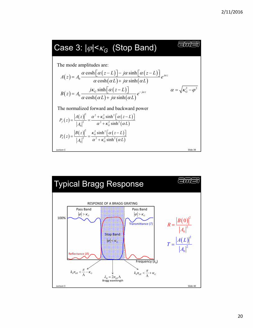
Typical Bragg Response

Lecture 5 Slide 40

100%

RESPONSE OF A BRAGG GRATING

Stop Band

Pass Band Pass Band

G G

G

0 eff Gk n

Frequency (k0)

0 eff Gk n

Reflectance (R)

Transmittance (T)

2

2

0

2

0

2

0

A LT

BR

A

A

eff2B n Bragg wavelength

2/11/2016

21

Non-Directional Coupling

Non-Directional Coupling

Lecture 5 42

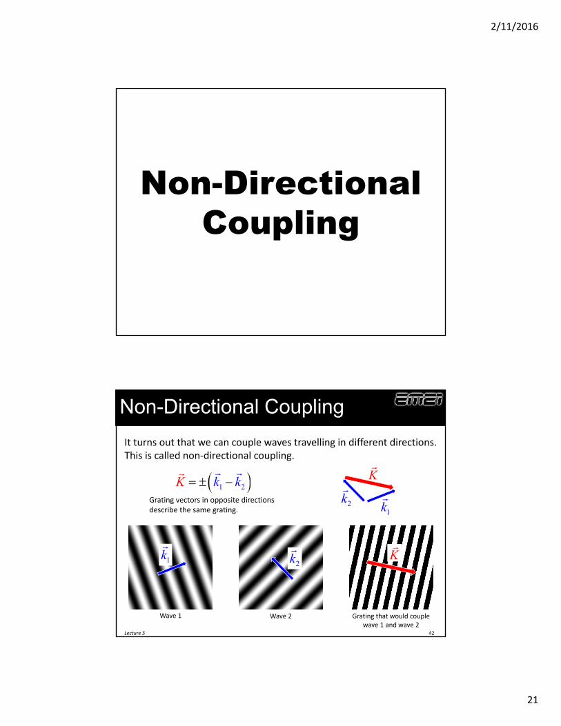
It turns out that we can couple waves travelling in different directions.  This is called non‐directional coupling.

2k

1k

K

1 2k kK

Wave 1 Wave 2 Grating that would couple wave 1 and wave 2

1k

2k

K

Grating vectors in opposite directions describe the same grating.

2/11/2016

22

Phase Matching with Gratings

Generalized Framework

Lecture 5 Slide 44

How do we couple two completely different modes so they can exchange power?  Ordinarily, this will not happen.

1

2

2/11/2016

23

Phase Matching

Lecture 5 Slide 45

We can couple any two modes using a grating.

1

2

K

The phase matching condition to couple energy between two modes is

1 2K 1

2

K

Grating Coupler Regimes

Lecture 5 Slide 46

Short period gratingsBragg gratingsContradirectional coupling

Long period gratingsCodirectional coupling

“Medium” period gratingsNon‐directional coupling

2/11/2016

24

Mode-Matching Vs.

Coupled-Wave

Frameworks to Model Propagation

Lecture 5 Slide 48

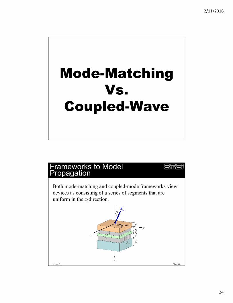
Both mode-matching and coupled-mode frameworks view devices as consisting of a series of segments that are uniform in the z-direction.

2/11/2016

25

Mode-Matching Framework (1 of 3)

Lecture 5 Slide 49

Mode matching views the field in a segment as being the sum of a set of orthogonal basis functions (eigen-modes).

+ + += +

m mm

E x a f x

E x 1f x 2f x 3f x 4f x mf x

Mode-Matching Framework (2 of 3)

Lecture 5 Slide 50

The modes within a segment accumulate phase differently as they propagate, but they do not interact and they propagate independently.

+

+

+

=

th

complete descriptionof the eigen-mode

, mj zm m

m

m

E x z a f x e

,E x z

11

j zf x e

22

j zf x e

33

j zf x e

44

j zf x e

2/11/2016

26

Mode-Matching Framework (3 of 3)

Lecture 5 Slide 51

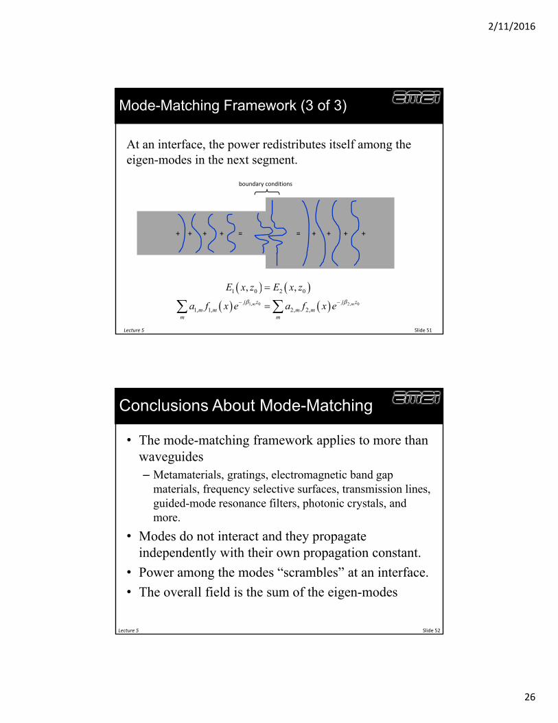
At an interface, the power redistributes itself among the eigen-modes in the next segment.

+ + + =+

1, 0 2, 0

1 0 2 0

1, 1, 2, 2,

, ,

m mj z j zm m m m

m m

E x z E x z

a f x e a f x e

+ + += +

boundary conditions

Conclusions About Mode-Matching

• The mode-matching framework applies to more than waveguides– Metamaterials, gratings, electromagnetic band gap

materials, frequency selective surfaces, transmission lines, guided-mode resonance filters, photonic crystals, and more.

• Modes do not interact and they propagate independently with their own propagation constant.

• Power among the modes “scrambles” at an interface.

• The overall field is the sum of the eigen-modes

Lecture 5 Slide 52

2/11/2016

27

Coupled-Wave Framework (1 of 3)

Lecture 5 Slide 53

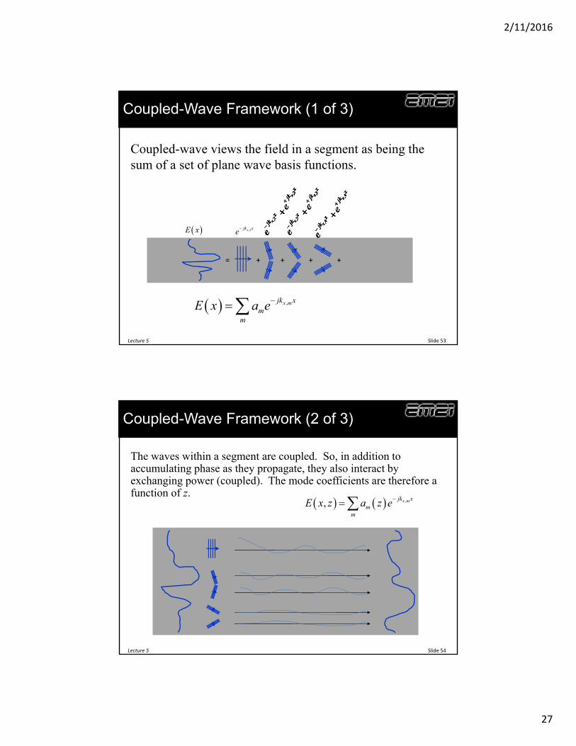
Coupled-wave views the field in a segment as being the sum of a set of plane wave basis functions.

+ + += +

,x mjk xm

m

E x a e

E x ,1xjk xe

Coupled-Wave Framework (2 of 3)

Lecture 5 Slide 54

The waves within a segment are coupled. So, in addition to accumulating phase as they propagate, they also interact by exchanging power (coupled). The mode coefficients are therefore a function of z.

,, x mjk xm

m

E x z a z e

2/11/2016

28

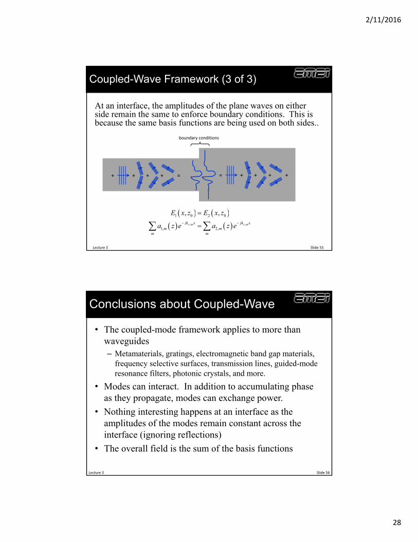
Coupled-Wave Framework (3 of 3)

Lecture 5 Slide 55

At an interface, the amplitudes of the plane waves on either side remain the same to enforce boundary conditions. This is because the same basis functions are being used on both sides..

+ + ++ =

boundary conditions

+ + += +

, ,

1 0 2 0

1, 2,

, ,

x m x mjk x jk xm m

m m

E x z E x z

a z e a z e

Conclusions about Coupled-Wave

• The coupled-mode framework applies to more than waveguides– Metamaterials, gratings, electromagnetic band gap materials,

frequency selective surfaces, transmission lines, guided-mode resonance filters, photonic crystals, and more.

• Modes can interact. In addition to accumulating phase as they propagate, modes can exchange power.

• Nothing interesting happens at an interface as the amplitudes of the modes remain constant across the interface (ignoring reflections)

• The overall field is the sum of the basis functions

Lecture 5 Slide 56

2/11/2016

29

How Do We Reconcile These Two Theories?

Lecture 5 57

Plane waves do not exist in inhomogeneous materials.

If we force them to exist, they exist in “sets” and the plane waves exchange energy as they propagate.

In this sense, we can think of modes as the set of plane waves that propagate independently of other sets of plane waves.

This transforms coupled‐mode framework to the mode‐matching frame work.