Lecture 6 Fourier Transform in N Dimensions 6.1 Learning Objectives • Develop an intuitive understanding for multidimensional spatial frequencies, and the N-D Fourier transform. • Recognize the typical appearance of N-D Fourier transforms, eg: the distribution of signal in the spatial frequency domain. • Recognize basic connections between features in the spatial domain versus the spa- tial frequency domain. 6.2 Introduction The extension of the FT to multi-dimensional signals enables us to analyze images (or higher-dimensional signals) in terms of a combination of multi-dimensional complex ex- ponentials (waves with various frequencies and ‘directions’). 6.3 Definition In the general case of an N-dimensional space, we consider a signal f (r), where r = [r 1 ,r 2 ,...,r N ] denotes a location in R N . The N-dimensional Fourier Transform (FT) of f (r) is defined as: ˆ f (u)= Z R N f (r)e -i2⇡r·u dr where r · u = r 1 u 1 + r 2 u 2 + ··· + r N u N is the dot product between vectors r and u. The corresponding inverse FT (iFT) is defined as: f (r)= Z R N ˆ f (u)e i2⇡r·u du 29
Transcript
Lecture 6
Fourier Transform in N Dimensions
6.1 Learning Objectives
• Develop an intuitive understanding for multidimensional spatial frequencies, andthe N-D Fourier transform.
• Recognize the typical appearance of N-D Fourier transforms, eg: the distribution ofsignal in the spatial frequency domain.
• Recognize basic connections between features in the spatial domain versus the spa-tial frequency domain.
6.2 Introduction
The extension of the FT to multi-dimensional signals enables us to analyze images (orhigher-dimensional signals) in terms of a combination of multi-dimensional complex ex-ponentials (waves with various frequencies and ‘directions’).
6.3 Definition
In the general case of an N-dimensional space, we consider a signal f(r), where r =[r1, r2, . . . , rN ] denotes a location in RN . The N-dimensional Fourier Transform (FT) off(r) is defined as:
f̂(u) =
Z
RN
f(r)e�i2⇡r·udr
where r · u = r1u1 + r2u2 + · · ·+ rNuN is the dot product between vectors r and u.The corresponding inverse FT (iFT) is defined as:
f(r) =
Z
RN
f̂(u)ei2⇡r·udu
29
30 LECTURE 6. FOURIER TRANSFORM IN N DIMENSIONS
Similar to the 1D FT case, the iFT expression above e↵ectively describes the decomposi-tion of our signal f(r) into a superposition of planar waves e�i2⇡r·u, where each of thesewaves has spatial frequency given by u. When combined to reconstruct f(r), each ofthese planar waves is scaled by a complex-valued amplitude given by f̂(u).
Using a slightly di↵erent notation, this expression can be reduced to the specific caseof a 2D image f(x, y):
f̂(u, v) =
Z
R2
f(x, y)e�i2⇡(xu+yv)dxdy
with corresponding iFT given by:
f(x, y) =
Z
R2
f̂(u, v)ei2⇡(xu+yv)dudv
6.4 A Few Common Fourier Transform Pairs
f(x, y) f̂(u, v)
�(x, y) 1
1 �(u, v)
�(x� x0, y � y0) e�i2⇡(ux0+vy0)
ei2⇡(xu0+yv0) �(u� u0, v � v0)
rect(x, y) sinc(u)sinc(v) = sin(⇡u)⇡u
sin(⇡v)⇡v
6.5 Interpretation and Examples
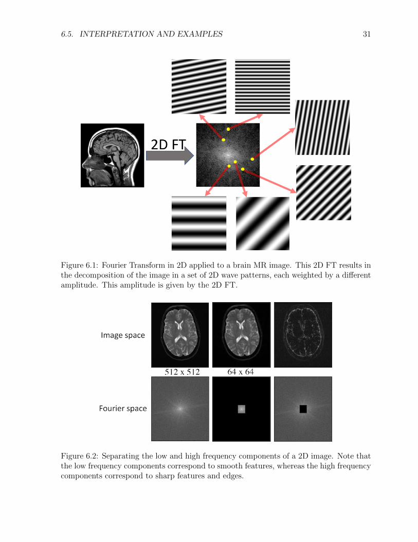
As illustrated in Figure 6.1, the 2D FT represents a 2D signal (an image) as a superpositionof 2D waves with di↵erent frequencies and orientations.
Additionally, the 2D FT enables insightful interpretations of the di↵erent 2D frequencyregions. For instance the low frequency regions (close to (u, v) = (0, 0)) represent smoothfeatures, whereas the high frequency regions represent sharp features and edges. This isillustrated in Figure 6.2.
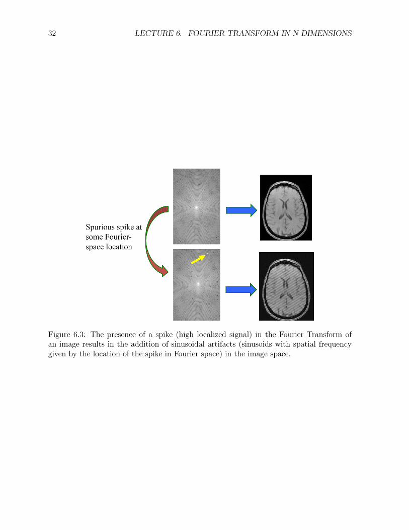
Finally, image artifacts are sometimes easy to interpret in Fourier space. An exampleof a spike artifact is shown in Figure 6.3.
6.5. INTERPRETATION AND EXAMPLES 31
Figure 6.1: Fourier Transform in 2D applied to a brain MR image. This 2D FT results inthe decomposition of the image in a set of 2D wave patterns, each weighted by a di↵erentamplitude. This amplitude is given by the 2D FT.
Figure 6.2: Separating the low and high frequency components of a 2D image. Note thatthe low frequency components correspond to smooth features, whereas the high frequencycomponents correspond to sharp features and edges.
32 LECTURE 6. FOURIER TRANSFORM IN N DIMENSIONS
Figure 6.3: The presence of a spike (high localized signal) in the Fourier Transform ofan image results in the addition of sinusoidal artifacts (sinusoids with spatial frequencygiven by the location of the spike in Fourier space) in the image space.