T.P. Zieliński Damped sinusoids PLC Lecture 7 / p.1

LECTURE 7: Damped sinusoids 7.1. RLC circuits Input volatage: u(t) (u(t) = 0 dla t < 0) Output voltage: uC(t) (on the capacitor) Fundamental relations: ic(t) =C⋅duC(t)/dt uL(t) =C⋅diL(t)/dt From Kirchhoff law:

( ) 1( ) ( ) ( ) ( ) ( ) ( )R L C

di tRi t L i t dt u t u t u t u tdt C

+ + = + + =∫ (*)

Assuption:

zero initial voltage on the capacitor

Fourier transform of both sides of (*):

( ) 1( ) ( ) ( )di tRi t L i t dt u t

dt C+ + =∫

1 ( ) ( )R j L I j U j

j C⎡ ⎤

+ ω + ω = ω⎢ ⎥ω⎣ ⎦

Only for the capacitance:

)()(1 tudttiC C=∫

)()(1ω=ω

ωjUjI

Cj C

T.P. Zieliński Damped sinusoids PLC Lecture 7 / p.2

Inout / output relation:

2

1( ) 1( ) 1( ) ( ) ( ) 1

CU j j CH jU j LC j RC jR j L

j C

ω ωωω ω ωω

ω

= = =+ ++ +

22

11( ) 1( ) ( ) 1 ( ) ( )

LCH j RLC j RC j j jL LC

ωω ω ω ω

= =+ + + +

After new denotations:

)2/()/(,1 00 ω=ξ=ω LRLC

we get standard transfer function of the resonant system:

( ) 12)/(1

2)()(

02

0200

2

20

+ωωξ+ωω−=

ω+ωξω+ω

ω=ω

jjjjH

Alternatively:

02

0120

21

21 ,1,

1,

)()( ξω=ξ−ω=ω

ξ−

ω=

ω+ω+ω

=ω aAjaAjH

Impulse response:

( )1sin ω dla 0

( )0 dla 0

atAe t th t

t

−⎧ ≥= ⎨

<⎩

( )0(ξω ) 20

02

ω sin ω 1 dla 0( ) 1

0 dla 0

te t th t

t

ξξ

−⎧ − ⋅ ≥⎪= −⎨⎪ <⎩

ω1 – pusation of the RLC system = attenuated oscillations (ω1 ≠ ω0 for ξ≠0) ω0 – eigen pusation of the un-attenuated system

T.P. Zieliński Damped sinusoids PLC Lecture 7 / p.3

0.01 0.1 1 10 100ω [rd/s]

-80

-60

-40

-20

0

20

20lo

g 10|H

(jω)|

[dB

]

Charakterystyka amplitudowa

0.01 0.1 1 10 100

ω [rd/s]

-200

-160

-120

-80

-40

0

Φ(jω

) [de

g]

Charakterystyka fazowa

0 10 20 30 40

t [s]

-0.4

-0.2

00.2

0.4

0.6

0.8

h(t)

Odpowiedź impulsowa

0 10 20 30 40

t [s]

0

0.25

0.50.75

1

1.25

1.5

u(t)

Odpowiedź skokowa

Maximum of |H(ω)| for ω = ω1 Two poles = decreasing 2 * -20 dB = -40 dB per decade.

|H(ω)| (magnitude) ∠H(ω) (angle)

Impulse response h(t) Step response u(t)

T.P. Zieliński Damped sinusoids PLC Lecture 7 / p.4

0 0.5 1 1.5 2 2.5 3

ω [rd/s]

0

1

2

3

4

5

6

|H(jω

)|Charakterystyka amplitudowa

ξ = 0,1

ξ = 0,3

ξ = 0,5

0 0.5 1 1.5 2 2.5 3

ω [rd/s]

-3

-2

-1

0

Φ(jω

) [rd

]

Charakterystyka fazowa

ξ = 0,5

ξ = 0,3

ξ = 0,1

0 10 20 30 40t [s]

-0.8-0.6-0.4-0.2

00.20.40.60.8

1

h(t)

Odpowiedź impulsowa

ξ = 0,3

ξ = 0,1

0 10 20 30 40

t [s]

00.20.40.60.8

11.21.41.61.8

u(t)

Odpowiedź skokowa

ξ = 0,3ξ = 0,1

|H(ω)| (magnitude) ∠H(ω) (angle)

Impulse response h(t) Step response u(t)

T.P. Zieliński Damped sinusoids PLC Lecture 7 / p.5

Fourier spectra:

1) Exponential signal :

ω+=ω↔

⎩⎨⎧

≥<

= − jajH

tet

tx at1)(

000

)(dladla

, (a>0)

Proof: ω+

=ω+−

==∞

ω+−∞

ω+−∞

ω−− ∫∫ jae

jadtedtee tjatjatjat 1

)(1

0

)(

0

)(

0

2) Sinusoidal with exponential envelope:

20

20

0 )()(

0sin00

)(ω+ω+

ω=ω↔

⎩⎨⎧

≥ω<

= − jaAjX

tdlatAetdla

tx at , (a>0)

Proof: 0 0( )0

0 0

1sin( ) [ ]2

j t j tat j t a j tAe t e dt A e e e dtj

∞ ∞ω − ω− − ω − + ωω = − =∫ ∫

[ ] [ ]0 0( ) ( )

0 02a j t a j tA e dt e dt

j

∞ ∞− + ω−ω − + ω+ω⎛ ⎞

= − =⎜ ⎟⎜ ⎟⎝ ⎠∫ ∫

( )

( )( )

( )0 0( ) ( )

0 0

1 10 02 ( ) ( )

a j t a j tA e ej a j a j

− + ω−ω − + ω+ω⎛ ⎞∞ ∞= − =⎜ ⎟⎜ ⎟− + ω − ω − + ω + ω⎝ ⎠

( )( ) ( ) 2

020

00

0

00 )()(2

2)(1

)(1

2 ω+ω+

ω=

ω+ω+ω−ω+ω

=⎟⎟⎠

⎞⎜⎜⎝

⎛ω+ω+

−ω−ω+

=jaA

jajaj

jA

jajajA

3) Sinusoidal with exponential envelope:

20

20 )(

)(0cos00

)(ω+ω+

ω+=ω↔

⎩⎨⎧

≥ω<

= − jajaAjX

ttAet

tx at dladla

, (a>0)

Proof: as above, setting cos(ω 0t) = 1/2(exp(jω 0t)+exp(−jω 0t)).

T.P. Zieliński Damped sinusoids PLC Lecture 7 / p.6

7.2. Hilbert transform method Continuous Hilbert transform of the real signal xr(t)

( ) [ ] ( )1( ) ( ) ( ) ( )ri r i r

xx t H x t d X j H j X j

t

π

−π

τ= = τ ↔ ω = ω ω

π − τ∫

xr(t) is convolved with 1( )π

h tt

= : (τ) () τ)( τrix x h tt d+∞

−∞

−= ∫

Inverse continuous Hilbert transform of the real signal xi(t)

( ) [ ] ( )1 11( ) ( ) ( ) ( )ir i r i

xx t H x t d X j H j X j

t

π− −

−π

τ= = − τ ↔ ω = ω ω

π − τ∫

xi(t) is convolved with 1( )π

h tt

= − : (τ) () τ)( τirx x h tt d+∞

−∞

−= ∫

T.P. Zieliński Damped sinusoids PLC Lecture 7 / p.7

Transfer functions:

Hilbert transform Inverse Hilbert transform phase shifter −π/2 phase shifter +π/2

( )

⎪⎩

⎪⎨

⎧

<ω=ω>ω−

=ω0000

j,,

j,jH

, ( )

⎪⎩

⎪⎨

⎧

<ω−=ω>ω

=ω−

0,0,00,

1

j

jjH

|H(jω)|

ω

1

|H-1(jω)|

ω

1

∠H(jω)

ω π/2

−π/2

∠H-1(jω)

ωπ/2

−π/2

Hilbert transform: xr(t) = cos(ω0t) ⇒ xi(t) = sin(ω0t) xr(t) = cos(ω0t)

( ) ( ) ( ) ( ) ( ) ( )tttttxi 0000 sin2/sinsin2/coscos2/cos)( ω=πω+πω=π−ω=

( ) ( ) ( ) ( ) ( ) ( )0 0 0 0( ) sin ω / 2 sin ω cos π / 2 cos ω sin π / 2 cos ωrx t t t t tπ= + = + =

Analytic signal:

Hilbert transform

xr(t) xr(t)

jxi(t)

x(t)=xr(t)+jxi(t)

xr(t)

jxi(t)

x(t)=xr(t)+jxi(t)

j

tj

ir etjttjxtxtx 0)sin()cos()()()( 00ω=ω+ω=+=

T.P. Zieliński Damped sinusoids PLC Lecture 7 / p.8

Derivation of Hilbert transfer function: Since (sgn = sign):

ω=ω↔=

jjXttx 2)()sgn()(

and Fourier transform has duality property: X(jt) ↔ 2πx(−ω) than

)sgn(2)sgn(2)(2)( ωπ−=ω−π=ω↔= jYjt

ty

Therefore:

1( ) ( ω) sgn(ω)π

h t H j jt

= ↔ = −

T.P. Zieliński Damped sinusoids PLC Lecture 7 / p.9

Fourier spectrum of the analytic signal:

( ) ( ) ( ) ( ) ( )( )txHjtxtxjtxtx rrir ⋅+=⋅+=

[ ]( ) ( ) ( ) ( ) ( )( ) 1 ( ) ( )rr i r rX j jH j X jX j jX j X j jH j X jω + ω = ω + + ωω ω =ω = ω

For ω ≥ 0:

[ ]( ) 2) )1 ) ( (( r rj j XX j X jj= − ωω + ω=

For ω < 0:

[ ]1 ( [1 1]) () )( 0( )rrj j X jX j Xj + ω= = − ω =ω

Example: Xr(jω)

ω

jXi(jω)

ω

X(jω)

ω

Having analytic signal x(t) we can reconstruct original signal xr(t) and its spectrum Xr(jω):

Since:

)()()( **

* ω−=⎥⎥⎦

⎤

⎢⎢⎣

⎡= ∫∫

∞+

∞−

ω∞+

∞−

ω− jXdtetxdtetx tjtj

therefore:

( ) ( ) ( ) ( ) ( ) ( )* *1 12 2r rx t x t x t X j X j X j⎡ ⎤ ⎡ ⎤= + ↔ ω = ω + − ω⎣ ⎦ ⎣ ⎦

( ) ( ) ( ) ( ) ( ) ( )* *1 12 2i ix t x t x t X j X j X j

j j⎡ ⎤ ⎡ ⎤= − ↔ ω = ω − − ω⎣ ⎦ ⎣ ⎦

T.P. Zieliński Damped sinusoids PLC Lecture 7 / p.10

Discrete Hilbert Transform = discrete convolution

( ) ( ) ( )) ( ( )i r Hk

H rk

x n x k h n k h k x n k∞

=−∞

∞

=−∞

−= − =∑ ∑

Impulse response from frequency response:

( )1( ) ,2

j j nh n H e e d nΩ Ω

−

= Ω − ∞ ≤ ≤ ∞∫π

ππ

Impulse response of discrete Hilbert filter ( Ω = 2πf/fs ):

∫π

π−

ΩΩ Ω= deeHnh njjHH )()(

⎥⎥⎦

⎤

⎢⎢⎣

⎡−

π=Ω−

π+Ω

π=

πΩ

π−

Ωπ

Ω

π−

Ω ∫∫0

0

0

0 112

)(21

21)( njnjnjnj

H ejn

ejn

jdejdjenh

[ ] [ ] [ ]nn

nn

eeeen

jnjnjj π−π

=π−π

=−−−π

= ππ− cos11cos222

1)()(2

1 00

Since:

22cos1sin2 α−

=α

Then finally:

( ) ( )

2/2/sin2/sin2)(

22

nn

nnnhH π

π=

ππ

=

( )

⎪⎩

⎪⎨⎧

=

≠π

π=

0,0

0,2/

2/sin)(

2

n

nn

nnhH

Multiplication with symmetrical window w(n):

( ) ( ) ( ) ( ), ,... 1,0,1,...,wH Hh n h n w n n M M= = − −

Delay M samples:

( ) ( ), 0,1,2,...,2wn Hb h n M n M= − =

y(n) x(n)

b2

b3

b1

b0

z−1

z−1

z−1

x(n−1)

x(n−2)

x(n−3)

T.P. Zieliński Damped sinusoids PLC Lecture 7 / p.11

Digital Hilbert filter ( ) ( ) ( ) ( )wH Hh n h n w n=

Solid line: M = 10 (N = 2M+1 = = 21). Dashed line: M = 20 (N = 2M+1 = 41) Ω = 2πf/fs with rectangular window with Blackman window

impulse response ( ) ( )wHh n

-10 -5 0 5 10

n

-0.6-0.4-0.2

00.20.40.6

h w(n

)

-10 -5 0 5 10

n

-0.6-0.4-0.2

00.20.40.6

h w(n

)

( ) j|H (e )|wH

Ω (magnitude)

0 0.1 0.2 0.3 0.4 0.5

Ω/2π [Hz/Hz]

00.20.40.60.8

11.2

|Hw

(ejΩ

)|

0 0.1 0.2 0.3 0.4 0.5

Ω/2π [Hz/Hz]

0

0.2

0.4

0.6

0.8

1

|Hw

(ejΩ

)|

( ) j|H (e )|wH

Ω (angle, phase)

0 0.1 0.2 0.3 0.4 0.5Ω/2π [Hz/Hz]

-180

-135

-90

-45

0

faza

Hw

(ejΩ

) [de

g]

0 0.1 0.2 0.3 0.4 0.5

Ω/2π [Hz/Hz]

-180

-135

-90

-45

0

faza

Hw

(ejΩ

) [de

g]

T.P. Zieliński Damped sinusoids PLC Lecture 7 / p.12

Hilbert transform calculation 1) In time as a convolution:

2 2

0

)

0

(( ) ( )( ) ( )M M

i rw

rk

kk

Hb hx n k x nk M kx n= =

− − −= =∑ ∑

2) In frequency via spectrum modification:

n = 0, 1, 2, ..., N−1, k = 0, 1, 2, ..., N−1, Ωk = k2π / N Xr(k) = Xr(ejΩk) Method 1 – imaginary complement

( ) ( )1

( ) ( )( ) ( ) ( ) ( )k k kkFFT N FFT Nj j jjrir ir X ex n X e H e X e x n

−ΩΩ Ω Ω⎯⎯⎯⎯→ → = ⎯⎯⎯⎯→

⎪⎪⎩

⎪⎪⎨

⎧

−==

−=−=

== Ω

)1)...(2/(,2/,0

)12/...(1,0,0

)()(

NNkjNk

Nkjk

eHkH kj

Method 2 – analytic signal (function hilbert() in Matlab)

( ) ( )1

( ) ( )( ) ( ) ( ) ( )k k kkFFT N FFT Nj jr r

j jrx n X X e x ne W e X e

−ΩΩ Ω Ω⎯⎯⎯⎯→ → = ⎯⎯⎯⎯→

⎪⎪⎩

⎪⎪⎨

⎧

−==

−==

== Ω

)1)...(2/(,02/,1

)12/...(1,20,1

)()(

NNkNk

Nkk

eWkW kj

X(jω)

ω

∠H(jω)

ωπ/2

−π/2

T.P. Zieliński Damped sinusoids PLC Lecture 7 / p.13

Hilbert transform applications 1) Instantaneous amplitude, phase, frequency demodulation:

Input: ( ) ( )cos( ( )), ( ) 0, ( )rx t A t t A t t= φ > φ − varying

After Hilbert: ( )( ) ( ) j tx t A t e φ=

Result: ( ) | ( ) |A t x t= , e.g. ( ) ?atA t e a−= → =

( )( )

Im ( )φ( ) tan

Re ( )x t

tx t

= e.g. 0 0φ(t)=ω φt +

φ( )ω( ) d ttdt

= e.g. [ ]0 0

0ω φ

ω( ) ω ?d t

tdt

+= = =

2) Instantaneous phase difference demodulation:

Input:

1 1 1( ) ( )cos( ( ))x t A t t t= ω + φ , A1(t)>0 slowly varying

2 2 2( ) ( )cos( ( ))x t A t t t= ω + φ , A1(t)>0 slowly varying

After Hilbert:

( )( )1

1 1( ) ( ) j t ty t A t e ω +φ= ,

( ) ( )( )ttjetAty 2)(22φ+ω=

( ) ( )( ) ( ) ( )( )1 2 2 1*

1 2 1 2 1 2( ) ( ) ( ) ( ) ( ) ( ) ( )j t t t t j t tz t y t y t A t A t e A t A t e−ω −φ +ω +φ φ −φ= = =

Result: ( ) ( ) ( ) ( )( )( )( ) ⎟⎟

⎠

⎞⎜⎜⎝

⎛=φ−φ=φΔ

tztzttt

realimagarctg12

In case of noisy signals:

( ) ( ) ( )*1 2( ) , ( ) 1

T T

T Tz t w y t y t d w d

− −

= τ + τ + τ τ τ τ =∫ ∫

T.P. Zieliński Damped sinusoids PLC Lecture 7 / p.14

Matlab program 1: amplitude and frequency demodulation N=1000; fpr=1000; dt=1/fpr; t=dt*(0:N-1); xr = (1+0.25*sin(2*pi*1*t)) .* cos(2*pi*(50*t+0.5*200*t.^2); x = hilbert(xr); ampl = abs(x); faza = unwrap(angle(x)); freq = 1/(2*pi)*diff(faza)./diff(t); plot(t,xr); pause plot(t,ampl); pause plot(t,faza); pause plot(t(1:N-1),freq); pause % ###################### % OUR Hilbert transform % modification 2 % ###################### Xr = fft(xr); PhaseMod = [ 0 -j*ones(1,Nx/2-1) 0 j*ones(1,Nx/2-1) ]; X = Xr .* PhaseMod; xi = ifft(X); xour = xr + j*xi; plot(t,xr,'r',t,xi,'b'); title('MY: RED=real, BLUE=imag'); grid; pause error = max(abs(x-xour)), pause % error in respect to Matab Matlab program 2: parameters of damped sinusoid % Parameters values fs =2000; % sampling freq [Hz] T = 2^4; % observation time [s] dt = 1/fs; % sepling pperiod [s] t = 0 : dt : L-dt; % discretized time N = length(t), % number of samples A0 = 4.5; % max (starting) amplitude d = 0.0001; % logarithmic decrement f0 = 32.77*(fs/N); % resonant frequency [Hz] w0 = 2*pi*f0; a = d*f0; % Signal generation x = A0* exp(-a*t) .* cos(2*pi*f0*t); % Add AWGN noise x = awgn(x,38); % SNR = 38 dB

T.P. Zieliński Damped sinusoids PLC Lecture 7 / p.15 y = hilbert(x); ylog = log(abs(y)); % Cut a fragment from the central part of y Nc = round(N/2+1); M=round(N/16); n = Nc - M : Nc + M; y = y(n); ylog = ylog(n); tn = t(n); subplot(111); stem(ylog); grid; pause % Estimate frequency phn = unwrap( atan2(imag(y),real(y)) ); fn = diff(phn)./diff(tn)/(2*pi); f0_est = mean(fn) % Estimate logarithmic decrement – attenuation speed p = polyfit(tn,ylog,1); d_est = -p(1)/f0_est disp('###################################################') err_f0 = 100*abs(f0-f0_est)/f0 err_d = 100*abs(d-d_est)/d disp('###################################################')

T.P. Zieliński Damped sinusoids PLC Lecture 7 / p.16

7.3. Fourier transform methods RLC circuit:

( )0(ξω ) 20

02

ω sin ω 1 dla 0( ) 1

0 dla 0

te t th t

t

ξξ

−⎧ − ⋅ ≥⎪= −⎨⎪ <⎩

Continuous signal model:

0

0( ) cos(2 () ( )) ZPDf t

wx t Ae tf ttδ εϕ επ−= + + +

εw(t) = AWGN,… εZPD(t) – Zero Point Drift (DC drift) Discrete signal model:

0[ ] cos( ) [ ] [ ]nw ZPDx n Ae n n nβ ϕω ε ε−= + + +

β = δf0/fs, ω0 = 2π(f0/fs)

Optimization = error minimization:

0

12

0 , ?00

( , , , , ) [ [ ] cos( ) ] minN

ndc dc

n

C A x n Ae n β ωβ ωβ ω ϕ ε ϕ ε

−−

==

= − + − ⎯⎯⎯→∑

Multiplication by a window:

)cos(][][][][ 0 ϕωβ +== − nAenwnxnwnv n (*)

N-point DFT (FFT) of v[k]:

1

0

2 , 0,1,2,[ ] [ ] , ..., 1k

Nj

nk

n k k NV vN

k n e ω πω−

−

=

= == −∑

0 0 5( 0.2) ,dN

dk πω < ≤= ±

For w[n] = rectangular window in (*):

⎟⎟⎠

⎞⎜⎜⎝

⎛

−−

+−

−= −

−− kk j

Nj

j

Nj

ee

eeAkV ω

ϕω

ϕ

λλ

λλ

*

*

11

11

2][

where: 0ωβλ je +−= , kNk )/2( πω = , “*” - complex conjugattion.

T.P. Zieliński Damped sinusoids PLC Lecture 7 / p.17

We assume that the spectral leakage from the negative frequencies can be neglected. Therefore in Duda-1 algorithm (Bertocco-Yoshida-1):

⎟⎟⎠

⎞⎜⎜⎝

⎛

−−

+−

−= −

−− kk j

Nj

j

Nj

ee

eeAkV ω

ϕω

ϕ

λλ

λλ

*

*

11

11

2][

⇓

⎟⎟⎠

⎞⎜⎜⎝

⎛

−−

≈ − kj

Nj

eeAkV ω

ϕ

λλ

11

2][

⇓ (max in V[k])

1 1

1 1

[ 1] [ ] 1 ,[ ] [ 1] 1

k k k

k k k

j j j

j j jV k V k e e eR r rV k V k e e e

ω ω ω

ω ω ω

λλ

+ −

− +

− − −

− − −

− − − − += = =

− + − − +

⇓

NjNjj

eRreRre k

/2/2 ππωλ

−−

= −

⇓ 0 Im{ln( )}ω λ= and Re{ln( )}β λ= − ⇓

0

002

,ssff f

fδ βω

π==

T.P. Zieliński Damped sinusoids PLC Lecture 7 / p.18

0

2( 1) [ ]cos[ ]

0, otherwise

Mm

wmM

A m m nw n N

π=

⎧ ⎛ ⎞−⎪ ⎜ ⎟= ⎝ ⎠⎨⎪⎩

∑

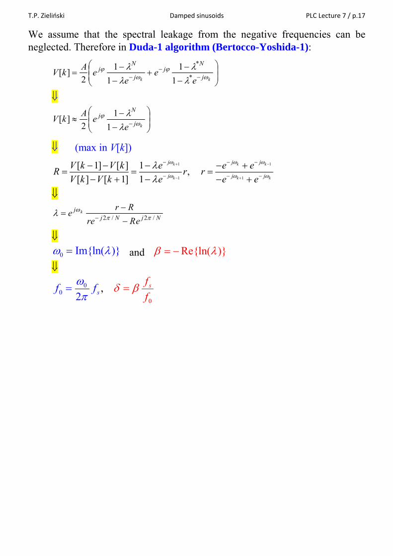
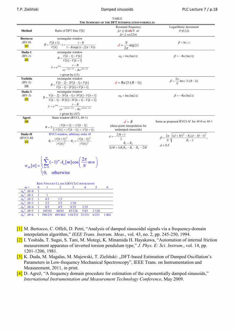
[1] M. Bertocco, C. Offeli, D. Petri, “Analysis of damped sinusoidal signals via a frequency-domain

interpolation algorithm,” IEEE Trans. Instrum. Meas., vol. 43, no. 2, pp. 245-250, 1994. [2] I. Yoshida, T. Sugai, S. Tani, M. Motegi, K. Minamida H. Hayakawa, “Automation of internal friction

measurement apparatus of inverted torsion pendulum type,” J. Phys. E: Sci. Instrum., vol. 14, pp. 1201-1206, 1981.

[3] K. Duda, M. Magalas, M. Majewski, T. Zieliński: „DFT-based Estimation of Damped Oscillation’s Parameters in Low-frequency Mechanical Spectroscopy”, IEEE Trans. on Instrumentation and Measurement, 2011, in print.

[4] D. Agrež, “A frequency domain procedure for estimation of the exponentially damped sinusoids,” International Instrumentation and Measurement Technology Conference, May 2009.

RIFE-VINCENT CLASS I (RVCI) COEFFICIENTS m = 0 1 2 3 4 5 6

Amw, M=0 1

Amw, M=1 1 1

Amw, M=2 1 4/3 1/3

Amw, M=3 1 3/2 3/5 1/10

Amw, M=4 1 8/5 4/5 8/35 1/35

Amw, M=5 1 105/63 60/63 45/126 5/63 1/126

Amw, M=6 1 396/231 495/462 110/231 33/231 6/231 1/462

TABLE THE SUMMARY OF THE DFT INTERPOLATION FORMULAS

Method Ratio of DFT bins V[k] Resonant frequency

f0= fs (k±d)/N or f0= fs ω0/(2π)

Logarithmic decrement δ=β fs/f0

Bertocco (BY-0)

[1]

rectangular window

][]1[

kVkV

R±

= ,))/2(exp(1

1NjR

Rzπ−±−

−=

arg{ }2

zd Nπ

=

||ln z=β

Duda-1 (BY-1)

[2]

rectangular window

]1[][][]1[

+−−−

=kVkV

kVkVR

NjNjj

eRreRre k

/2/2 ππωλ

−−

=−

r given by (13)

)}Im{ln(0 λω =

)}Re{ln(λβ −=

Yoshida (BY-2)

[3]

rectangular window

]1[][2]1[][]1[2]2[

++−−+−−−

=kVkVkV

kVkVkVR

Re{3/( 1)}d R= − )}1/(3Im{2

−−= RNπβ

Duda-3 (BY-3)

[2]

rectangular window

]2[]1[3][3]1[]1[][3]1[3]2[

+−++−−+−+−−−

=kVkVkVkVkVkVkVkVR

)/2(2)/2(2 NjNjj

eRreRre k

ππωλ

−−

=−

r given by (A7)

)}Im{ln(0 λω =

)}Re{ln(λβ −=

Agrež [4]

Hann window (RVCI, M=1)

|]1[||]1[||][|2|]1[||]1[|2

++−+−−+

=kVkVkV

kVkVR

d R=

(three-point interpolation for undamped sinusoids)

Same as proposed RVCI-M for M=0 or M=1

Duda-M (RVCI-M)

[2]

RVCI window, arbitrary order M

2

2

1 |][||]1[|

kVkVR +

= , 2

2

2 |][||]1[|

kVkVR −

=

MRRRRMRR

Md

2)1(2

212

2121

21

−−−+−

+−=

5.0

,1

)1()(2

1

21

2

≠

−−−−+

=

dR

MdRMdNπβ

T.P. Zieliński Damped sinusoids PLC Lecture 7 / p.19

Matlab program 3: parameters of damped sinusoid via IpDFT format long % Parameters values …the same as in program2 % Signal generation ….the same as in program2 % Add AWGN noise…the same as in program2 % Yoshida 1981 - FFT with rectangular window Y = fft(x,N)/N; % FFT [Ymax s]=max(abs(Y)); % find maximum Y = Y/Ymax; % if( abs(Y(s-1)) > abs(Y(s+1)) ) ss=s-1; else ss=s; end % Real maximum should be between freq samples 2<=no<3 s1=ss-1; s2=ss; s3=s2+1; s4=s3+1; R=(Y(s1)-2*Y(s2)+Y(s3))/(Y(s2)-2*Y(s3)+Y(s4)); d_est1 = 2*pi*(imag(-3/(R-1))./real((s1-1)-3/(R-1))); f_est1 =(fs/N)*real((s1-1)-3/(R-1); err_d1 = 100*abs(d-d_est1 )/d; err_f1 = 100*(f0 - f_est)/f; % Agres 2009: FFT with Hanning window w = hanning(N)'; Yw = fft(w.*x,NFFT)/NFFT; % FFT(signal*window) Yw = abs(Yw); % [Ywmax sw]=max(Yw); % find maximum Yw = Yw/Ywmax; % scale % Yw can be calculated from Y (Yoshida metod) by local smoothing [1/4, 1/2, 1/4] s1w = sw-1, s2w = sw, s3w = sw+1, Y1w = Yw(s1w), Y2w = Yw(s2w), Y3w = Yw(s3w), R = 2*( Y3w - Y1w ) / ( Y1w + 2*Y2w + Y3w ), pause d_est2 = R; k_est2 = (sw-1) + delta; f_est2 = f0*k_est2; err_d2 = 100*(d - d_est2)/d; err_f2 = 100*(f0 - f_est2)/f;

T.P. Zieliński Damped sinusoids PLC Lecture 7 / p.20

7.4. LS and Prony methods Design of AR (IIR) digital FILTER

- its impulse response is equal to x(n) - its frequency response fits to signal spectrum

- its parameters parameters of damped sinusoids

H(z) x(n)δ(n) y(n)

Dirac impulse

y(n) δ(n)

−a3

−a2

−a1y(n−1)

z−1

z−1

z−1

y(n−3)

y(n−2)

When ( ) ( )y n x n≈ ⇒ 1

( ) ( ) ( )N

kk

x n n a x n kδ=

= − −∑ linear self-prediction

Transfer function of digital filter:

1 2 1 1 11 2 1 2

1

1 1 1( )1 ... (1 )(1 )...(1 )1

N Nk N N

kk

H za z a z a z p z p z p za z

− − − − − −−

=

= = =+ + + + − − −+ ∑

For 2

s

fjfjz e e

πΩ= = H(z) → H(f).

Task: find poles of the transfer function for a given signal x(n)

2φ

k

k s

fjj f

k k kp r e r eπ

= ⋅ = ⋅ ⇒ ( )( ) nk kh n p=

( ) ( )/ 2 / 2 / 2

φ φ*

1 1 1

( ) 2 cos 2k k

N N Nnn j n j nn n n kk k k k k

k k k s

fx n p p r e r e r nf

π−

= = =

⎡ ⎤⎛ ⎞⎡ ⎤ ⎡ ⎤= + = ⋅ + ⋅ = ⋅⎢ ⎥⎜ ⎟⎣ ⎦⎢ ⎥⎣ ⎦ ⎝ ⎠⎣ ⎦∑ ∑ ∑

( )/ 2

ln( ) k

1

φ( ) 2 cos φ , ln( ),2

k

Nr n

k k k k sk

x n e n a r f fπ=

⎡ ⎤= ⋅ = − =⎣ ⎦∑

1

( ) ( ) ( )N

kk

y n n a y n kδ=

= − −∑

T.P. Zieliński Damped sinusoids PLC Lecture 7 / p.21

Linear self-prediction:

=Ax 0 , A – matrix with Toeplitz structure

=Xa 0 , X – matrix with Hankel structure

=Xa x , X – matrix with Hankel structure ALGORITH:

1) Solve the above equation in respect to a.

2) Find roots of pk polynomial having coeffs a. 3) Knowing pk calculate parameters of damped sins

2

φ kφln( ),2

k

k s

fjj f

k k k k k k sp r e r e a r f fπ

π= ⋅ = ⋅ ⇒ = − =

( )/ 2

ln( ) k

1

φ( ) 2 cos φ , ln( ),2

k

Nr n

k k k k sk

x n e n a r f fπ=

⎡ ⎤= ⋅ = − =⎣ ⎦∑

cos 2ka n k

s

fe nf

π− ⎛ ⎞⎜ ⎟⎝ ⎠

T.P. Zieliński Damped sinusoids PLC Lecture 7 / p.22

% LS solution of the AR filter of the second order (x is vertical) xm0 = x(3:end-0); xm1 = x(2:end-1); xm2 = x(1:end-2); a = [ -xm1(:) –xm2(:) ] \ xm0(:); % find LS solution r = roots([1 a(1) a(2)]); a_LS_est = abs(r(1)); d_LS_est = -log( a_est ); d_LS_est = d_LS_est*(length(x)-1)/f0/t(length(x)); % scaling f_LS_est = fs*angle(p)/(2*pi); % Prony solution – find AR filter of the second order corresponding to x(n) [b,a] = prony(x,1,2); % printsys(b,a,'z') [z,p,K] = TF2ZPK(b,a); % {a,b} {zeros, poles} a_est = abs(p(1)); d_est = -log( a_est ); d_est = d_est*(length(x)-1)/f0/t(length(x)); % scaling f_est = fs*angle(p)/(2*pi); % CHECK CORRECTNESS!

T.P. Zieliński Damped sinusoids PLC Lecture 7 / p.23

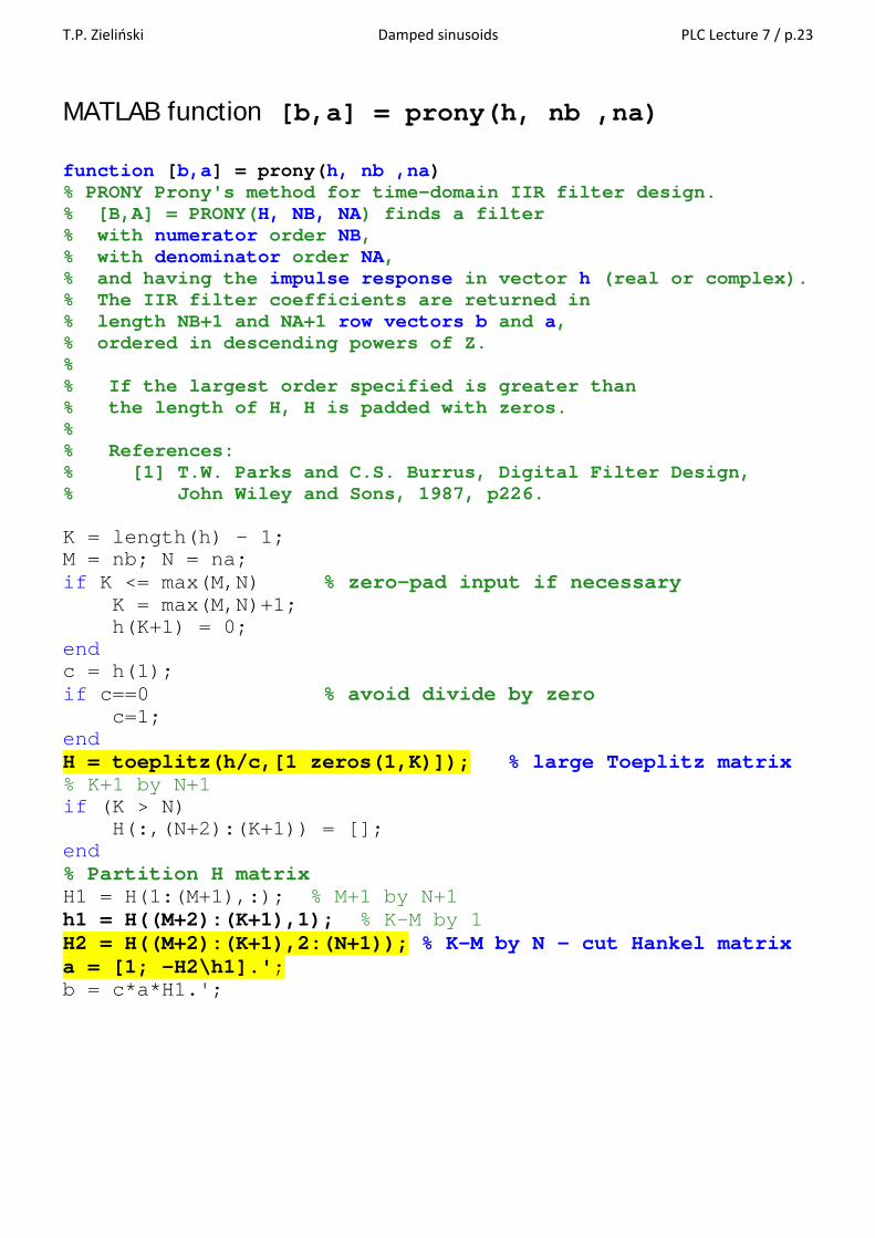
MATLAB function [b,a] = prony(h, nb ,na) function [b,a] = prony(h, nb ,na) % PRONY Prony's method for time-domain IIR filter design. % [B,A] = PRONY(H, NB, NA) finds a filter % with numerator order NB, % with denominator order NA, % and having the impulse response in vector h (real or complex). % The IIR filter coefficients are returned in % length NB+1 and NA+1 row vectors b and a, % ordered in descending powers of Z. % % If the largest order specified is greater than % the length of H, H is padded with zeros. % % References: % [1] T.W. Parks and C.S. Burrus, Digital Filter Design, % John Wiley and Sons, 1987, p226. K = length(h) - 1; M = nb; N = na; if K <= max(M,N) % zero-pad input if necessary K = max(M,N)+1; h(K+1) = 0; end c = h(1); if c==0 % avoid divide by zero c=1; end H = toeplitz(h/c,[1 zeros(1,K)]); % large Toeplitz matrix % K+1 by N+1 if (K > N) H(:,(N+2):(K+1)) = []; end % Partition H matrix H1 = H(1:(M+1),:); % M+1 by N+1 h1 = H((M+2):(K+1),1); % K-M by 1 H2 = H((M+2):(K+1),2:(N+1)); % K-M by N – cut Hankel matrix a = [1; -H2\h1].'; b = c*a*H1.';

T.P. Zieliński Damped sinusoids PLC Lecture 7 / p.24

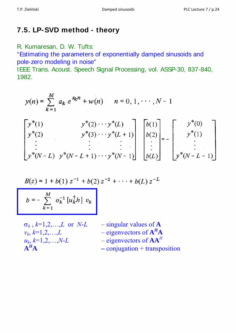
7.5. LP-SVD method - theory R. Kumaresan, D. W. Tufts: “Estimating the parameters of exponentially damped sinusoids and pole-zero modeling in noise” IEEE Trans. Acoust. Speech Signal Processing, vol. ASSP-30, 837-840, 1982.

σk , k=1,2,…,L or N-L – singular values of A vk, k=1,2,…,L – eigenvectors of AHA uk, k=1,2,…,N-L – eigenvectors of AAH AHA – conjugation + transposition

T.P. Zieliński Damped sinusoids PLC Lecture 7 / p.25

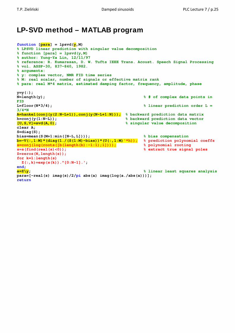
LP-SVD method – MATLAB program function [para] = lpsvd(y,M) % LPSVD linear prediction with singular value decomposition % function [para] = lpsvd(y,M) % author: Yung-Ya Lin, 12/11/97 % reference: R. Kumaresan, D. W. Tufts IEEE Trans. Acoust. Speech Signal Processing % vol. ASSP-30, 837-840, 1982. % arguments: % y: complex vector, NMR FID time series % M: real scalar, number of signals or effective matrix rank % para: real M*4 matrix, estimated damping factor, frequency, amplitude, phase y=y(:); N=length(y); % # of complex data points in FID L=floor(N*3/4); % linear prediction order L = 3/4*N A=hankel(conj(y(2:N-L+1)),conj(y(N-L+1:N))); % backward prediction data matrix h=conj(y(1:N-L)); % backward prediction data vector [U,S,V]=svd(A,0); % singular value decomposition clear A; S=diag(S); bias=mean(S(M+1:min([N-L,L]))); % bias compensation b=-V(:,1:M)*(diag(1./(S(1:M)-bias))*(U(:,1:M)'*h)); % prediction polynomial coeffs s=conj(log(roots([b(length(b):-1:1);1]))); % polynomial rooting s=s(find(real(s)<0)); % extract true signal poles Z=zeros(N,length(s)); for k=1:length(s) Z(:,k)=exp(s(k)).^[0:N-1].'; end; a=Z\y; % linear least squares analysis para=[-real(s) imag(s)/2/pi abs(a) imag(log(a./abs(a)))]; return