Lecture 7

Flow over immersed bodies.

Boundary layer.

Analysis of inviscid flow.

Flow over immersed bodies

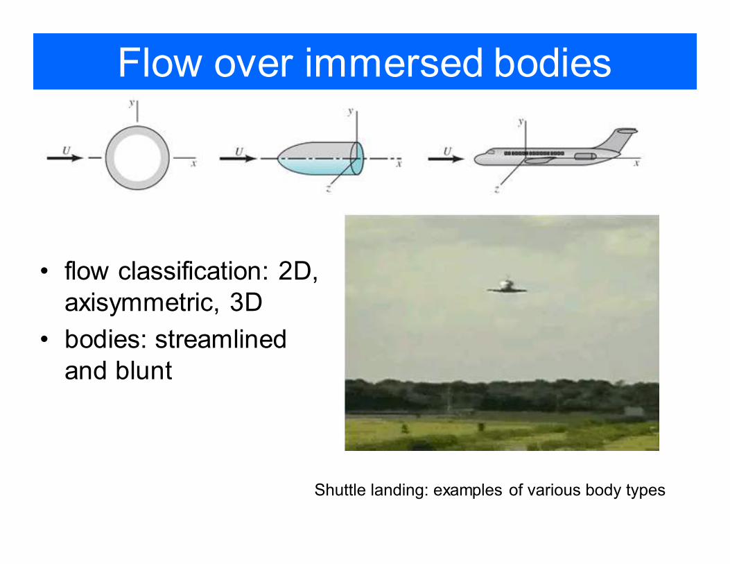
• flow classification: 2D,

axisymmetric, 3D

• bodies: streamlined

and blunt

Shuttle landing: examples of various body types

Lift and Drag

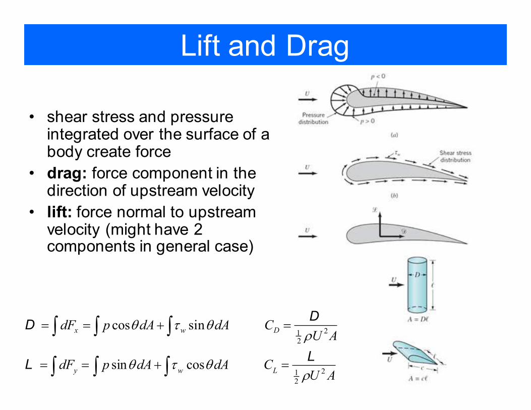
• shear stress and pressure integrated over the surface of a body create force

• drag: force component in the direction of upstream velocity

• lift: force normal to upstream velocity (might have 2 components in general case)

212

212

cos sin

sin cos

x w D

y w L

dF p dA dA CU A

dF p dA dA CU A

θ τ θρ

θ τ θρ

= = + =

= = + =

∫ ∫ ∫

∫ ∫ ∫

DD

LL

Flow past an object

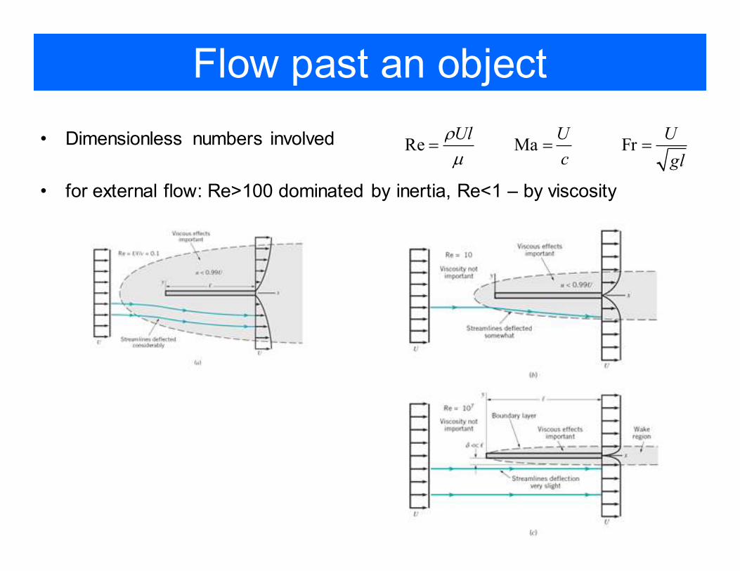
• Dimensionless numbers involved Re Ma FrUl U U

c gl

ρµ

= = =

• for external flow: Re>100 dominated by inertia, Re<1 – by viscosity

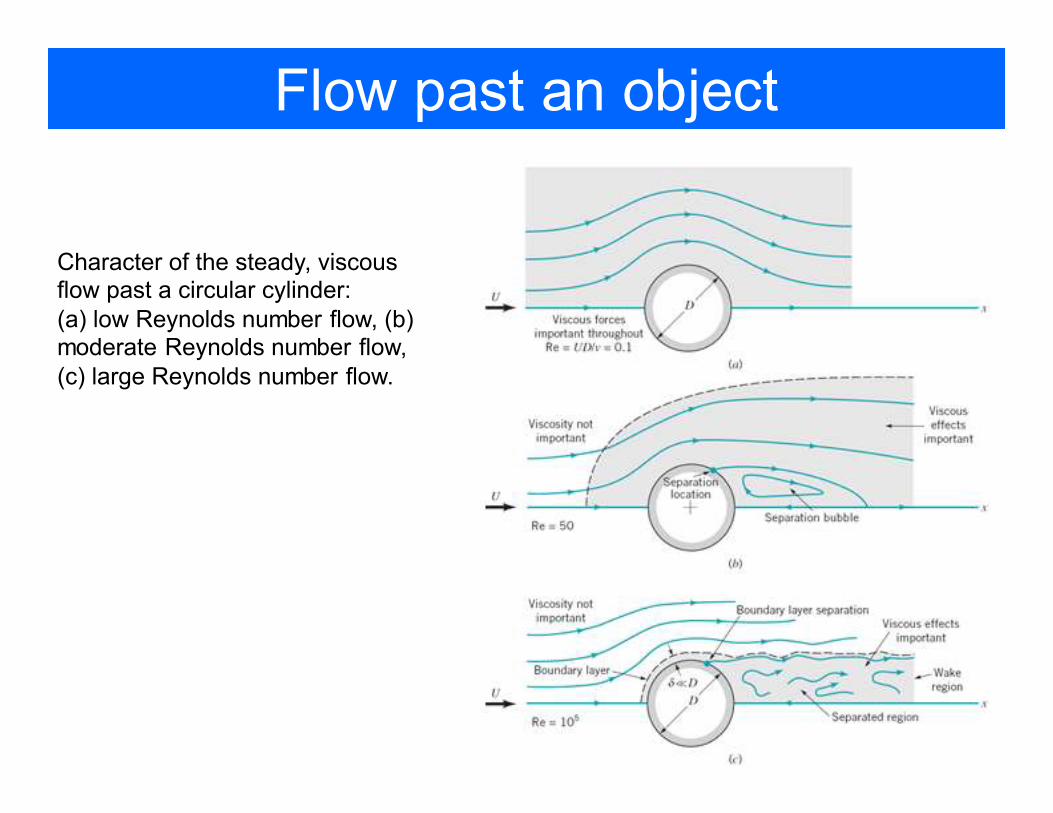
Flow past an object

Character of the steady, viscous flow past a circular cylinder:

(a) low Reynolds number flow, (b) moderate Reynolds number flow,

(c) large Reynolds number flow.

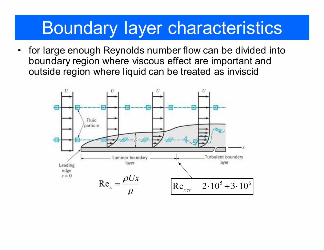
Boundary layer characteristics• for large enough Reynolds number flow can be divided into

boundary region where viscous effect are important and outside region where liquid can be treated as inviscid

Rex

Uxρµ

= 5 6Re 2 10 3 10xcr

⋅ ÷ ⋅�

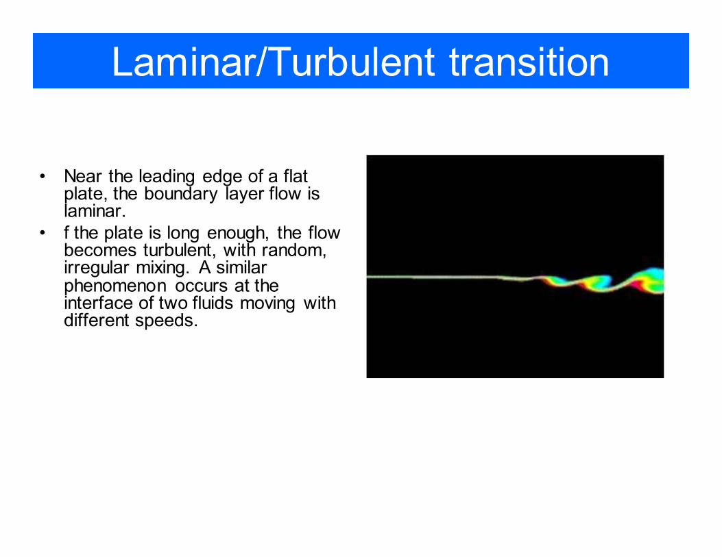
Laminar/Turbulent transition

• Near the leading edge of a flat plate, the boundary layer flow is laminar.

• f the plate is long enough, the flow becomes turbulent, with random, irregular mixing. A similar phenomenon occurs at the interface of two fluids moving with different speeds.

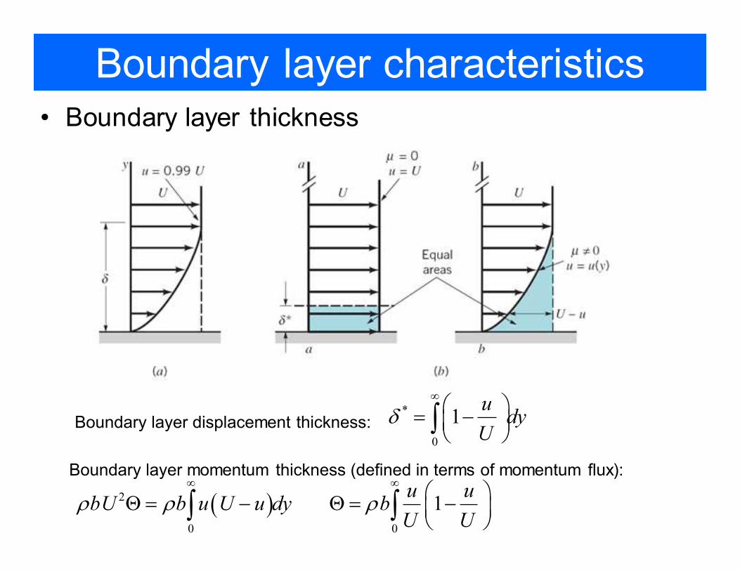
Boundary layer characteristics

• Boundary layer thickness

Boundary layer displacement thickness:*

0

1udy

Uδ

∞ = − ∫

Boundary layer momentum thickness (defined in terms of momentum flux):

( )2

0 0

1u u

bU b u U u dy bU U

ρ ρ ρ∞ ∞

Θ = − Θ = − ∫ ∫

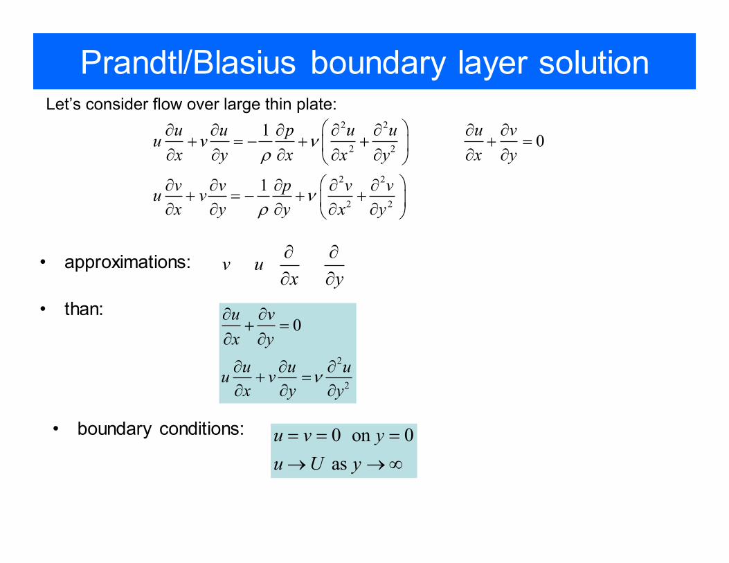
Prandtl/Blasius boundary layer solution

• approximations:

2 2

2 2

2 2

2 2

10

1

u u p u u u vu vx y x x y x y

v v p v vu vx y y x y

νρ

νρ

∂ ∂ ∂ ∂ ∂ ∂ ∂+ = − + + + =

∂ ∂ ∂ ∂ ∂ ∂ ∂

∂ ∂ ∂ ∂ ∂+ = − + + ∂ ∂ ∂ ∂ ∂

v ux y

∂ ∂∂ ∂

� �

2

2

0u v

x y

u u uu vx y y

ν

∂ ∂+ =

∂ ∂

∂ ∂ ∂+ =

∂ ∂ ∂

• than:

• boundary conditions: 0 on 0

as

u v y

u U y

= = =

→ → ∞

Let’s consider flow over large thin plate:

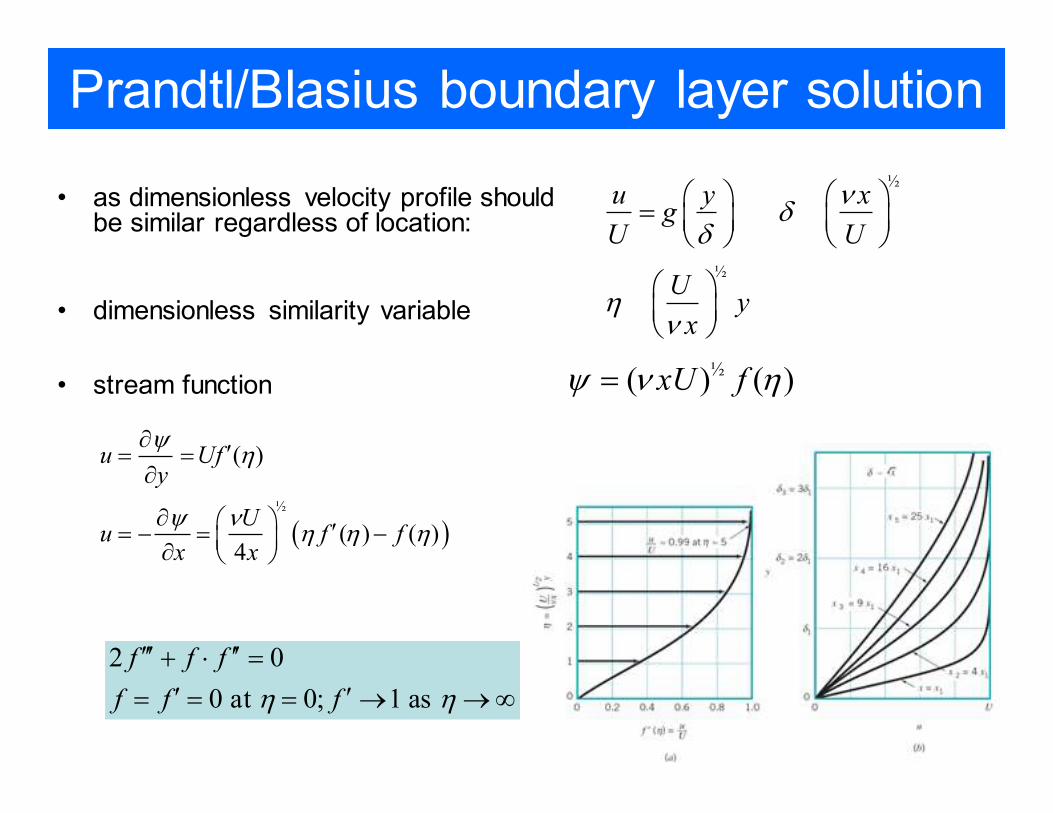
Prandtl/Blasius boundary layer solution

• as dimensionless velocity profile should be similar regardless of location:

½u y x

gU U

νδ

δ =

�

• dimensionless similarity variable

½U

yx

ην

�

• stream function ½( ) ( )xU fψ ν η=

( )½

( )

( ) ( )4

u Ufy

Uu f f

x x

ψη

ψ νη η η

∂′= =

∂

∂ ′= − = − ∂

2 0

0 at 0; 1 as

f f f

f f fη η

′′′ ′′+ ⋅ =

′ ′= = = → → ∞

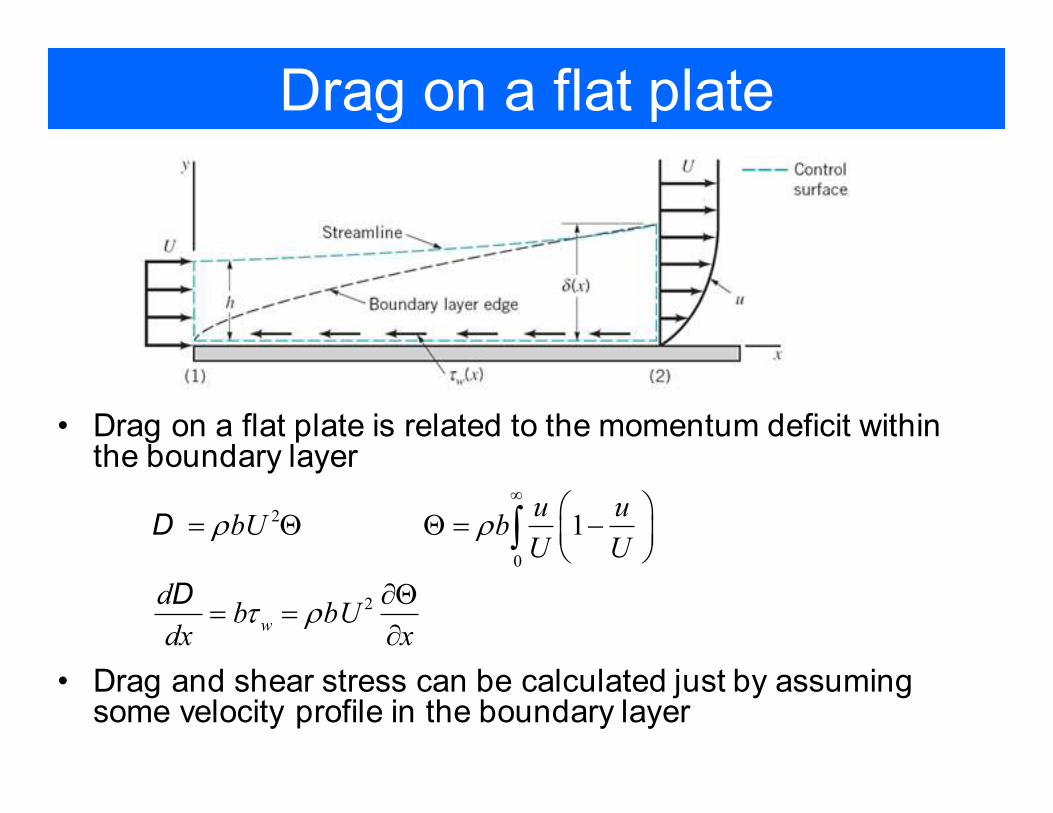
Drag on a flat plate

• Drag on a flat plate is related to the momentum deficit within the boundary layer

2

0

2

1

w

u ubU b

U U

db bU

dx x

ρ ρ

τ ρ

∞

= Θ Θ = −

∂Θ= =

∂

∫D

D

• Drag and shear stress can be calculated just by assuming some velocity profile in the boundary layer

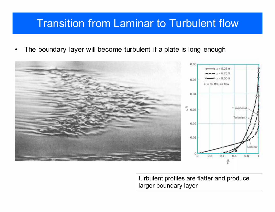
Transition from Laminar to Turbulent flow

• The boundary layer will become turbulent if a plate is long enough

turbulent profiles are flatter and produce larger boundary layer

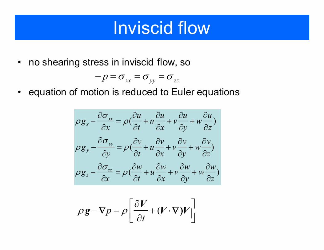
Inviscid flow

• no shearing stress in inviscid flow, so

xx yy zzp σ σ σ− = = =

• equation of motion is reduced to Euler equations

( )

( )

( )

xxx

yy

y

zzz

u u u ug u v w

x t x y z

v v v vg u v w

y t x y z

w w w wg u v w

x t x y z

σρ ρ

σρ ρ

σρ ρ

∂ ∂ ∂ ∂ ∂− = + + +

∂ ∂ ∂ ∂ ∂

∂ ∂ ∂ ∂ ∂− = + + +

∂ ∂ ∂ ∂ ∂

∂ ∂ ∂ ∂ ∂− = + + +

∂ ∂ ∂ ∂ ∂

(pt

ρ ρ∂

− = + ⋅ ∂

Vg V V∇ ∇)∇ ∇)∇ ∇)∇ ∇)

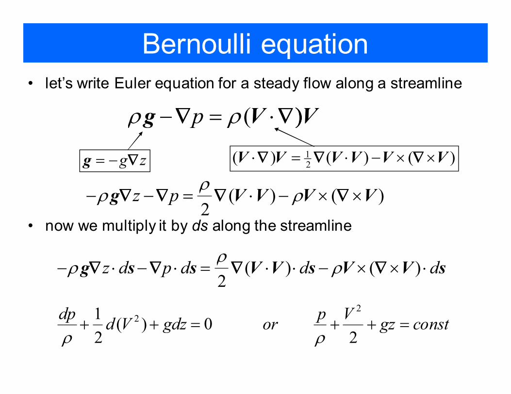
Bernoulli equation

• let’s write Euler equation for a steady flow along a streamline

(pρ ρ− = ⋅g V V∇ ∇)∇ ∇)∇ ∇)∇ ∇)

g z= − ∇∇∇∇g12

( ) ( ) ( )⋅ = ⋅ − × ×V V V V V V∇ ∇ ∇∇ ∇ ∇∇ ∇ ∇∇ ∇ ∇

( ) ( )2

z pρ

ρ ρ− − = ⋅ − × ×g V V V V∇ ∇ ∇ ∇∇ ∇ ∇ ∇∇ ∇ ∇ ∇∇ ∇ ∇ ∇

• now we multiply it by ds along the streamline

( ) ( )2

z d p d d dρ

ρ ρ− ⋅ − ⋅ = ⋅ ⋅ − × × ⋅g s s V V s V V s∇ ∇ ∇ ∇∇ ∇ ∇ ∇∇ ∇ ∇ ∇∇ ∇ ∇ ∇

221

( ) 02 2

dp p Vd V gdz or gz const

ρ ρ+ + = + + =

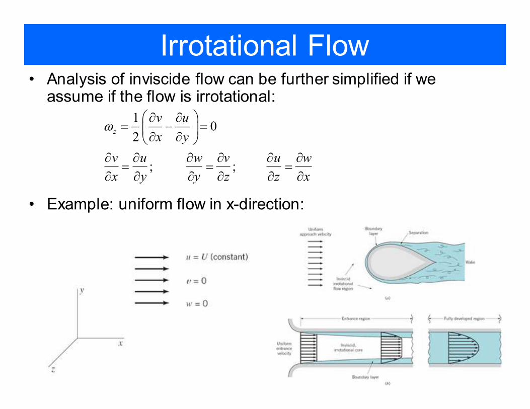
Irrotational Flow• Analysis of inviscide flow can be further simplified if we

assume if the flow is irrotational:

10

2

; ;

z

v u

x y

v u w v u w

x y y z z x

ω ∂ ∂

= − = ∂ ∂ ∂ ∂ ∂ ∂ ∂ ∂

= = =∂ ∂ ∂ ∂ ∂ ∂

• Example: uniform flow in x-direction:

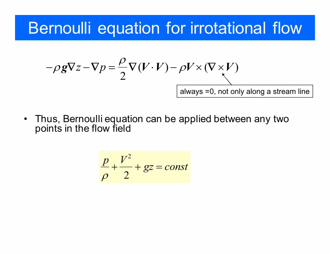
Bernoulli equation for irrotational flow

• Thus, Bernoulli equation can be applied between any two points in the flow field

( ) ( )2

z pρ

ρ ρ− − = ⋅ − × ×g V V V V∇ ∇ ∇ ∇∇ ∇ ∇ ∇∇ ∇ ∇ ∇∇ ∇ ∇ ∇

always =0, not only along a stream line

2

2

p Vgz const

ρ+ + =

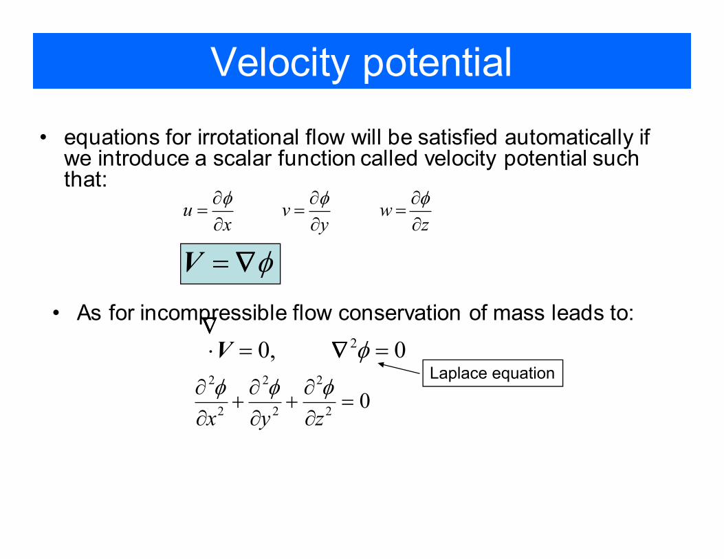
Velocity potential

• equations for irrotational flow will be satisfied automatically if we introduce a scalar function called velocity potential such that:

u v wx y z

φ φ φ∂ ∂ ∂= = =

∂ ∂ ∂

φ=V ∇∇∇∇

• As for incompressible flow conservation of mass leads to:

20, 0φ⋅ = =∇∇∇∇ V ∇∇∇∇Laplace equation2 2 2

2 2 20

x y z

φ φ φ∂ ∂ ∂+ + =

∂ ∂ ∂

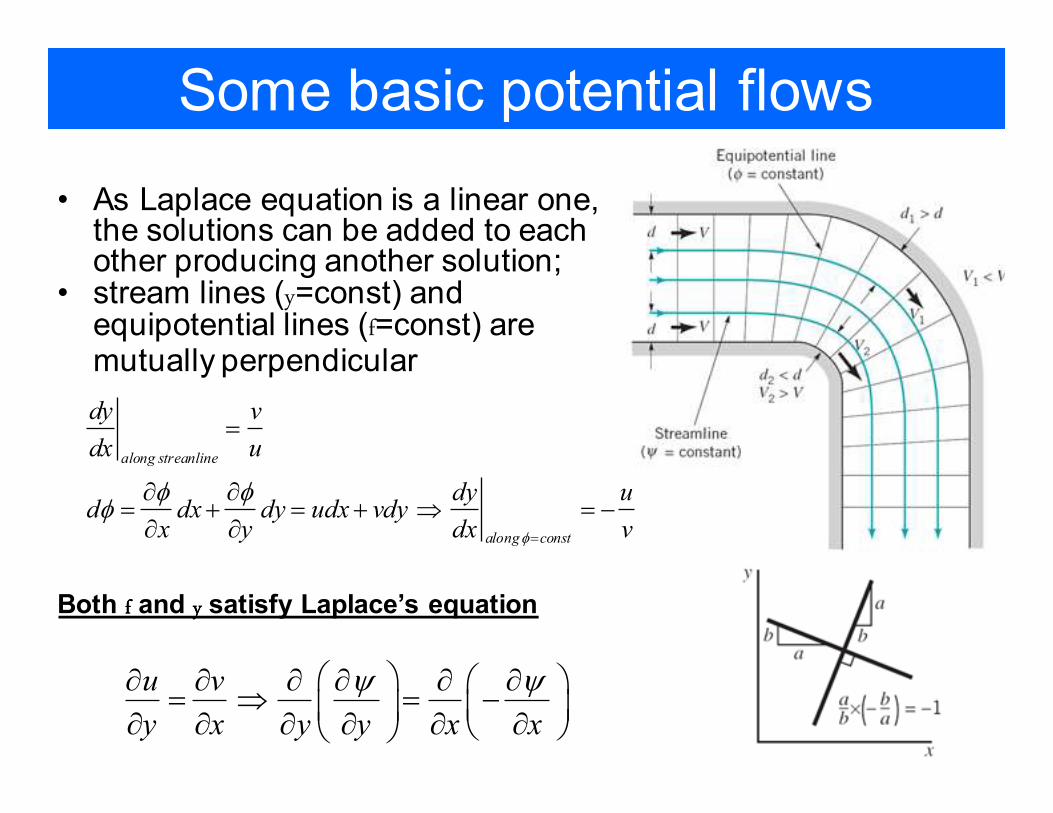
Some basic potential flows

• As Laplace equation is a linear one, the solutions can be added to each other producing another solution;

• stream lines (y=const) and equipotential lines (f=const) are mutually perpendicular

along streanline

along const

dy v

dx u

dy ud dx dy udx vdy

x y dx vφ

φ φφ

=

=

∂ ∂= + = + ⇒ = −

∂ ∂

Both ffff and yyyy satisfy Laplace’s equation

u v

y x y y x x

ψ ψ ∂ ∂ ∂ ∂ ∂ ∂ = ⇒ = − ∂ ∂ ∂ ∂ ∂ ∂

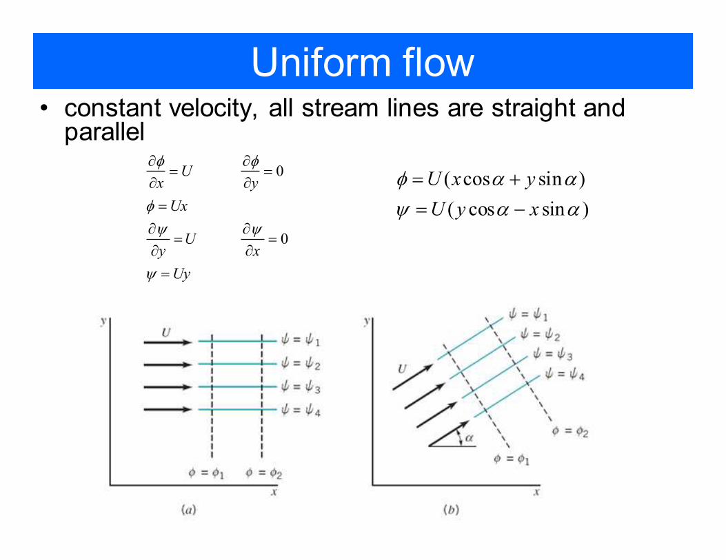
Uniform flow• constant velocity, all stream lines are straight and parallel

0

0

Ux y

Ux

Uy x

Uy

φ φ

φψ ψ

ψ

∂ ∂= =

∂ ∂

=

∂ ∂= =

∂ ∂

=

( cos sin )

( cos sin )

U x y

U y x

φ α α

ψ α α

= +

= −

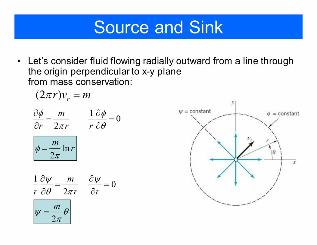
Source and Sink

• Let’s consider fluid flowing radially outward from a line through the origin perpendicular to x-y planefrom mass conservation:

(2 ) rr v mπ =

10

2

m

r r r

φ φπ θ

∂ ∂= =

∂ ∂

10

2

m

r r r

ψ ψθ π

∂ ∂= =

∂ ∂

ln2

mrφ

π=

2

mψ θ

π=

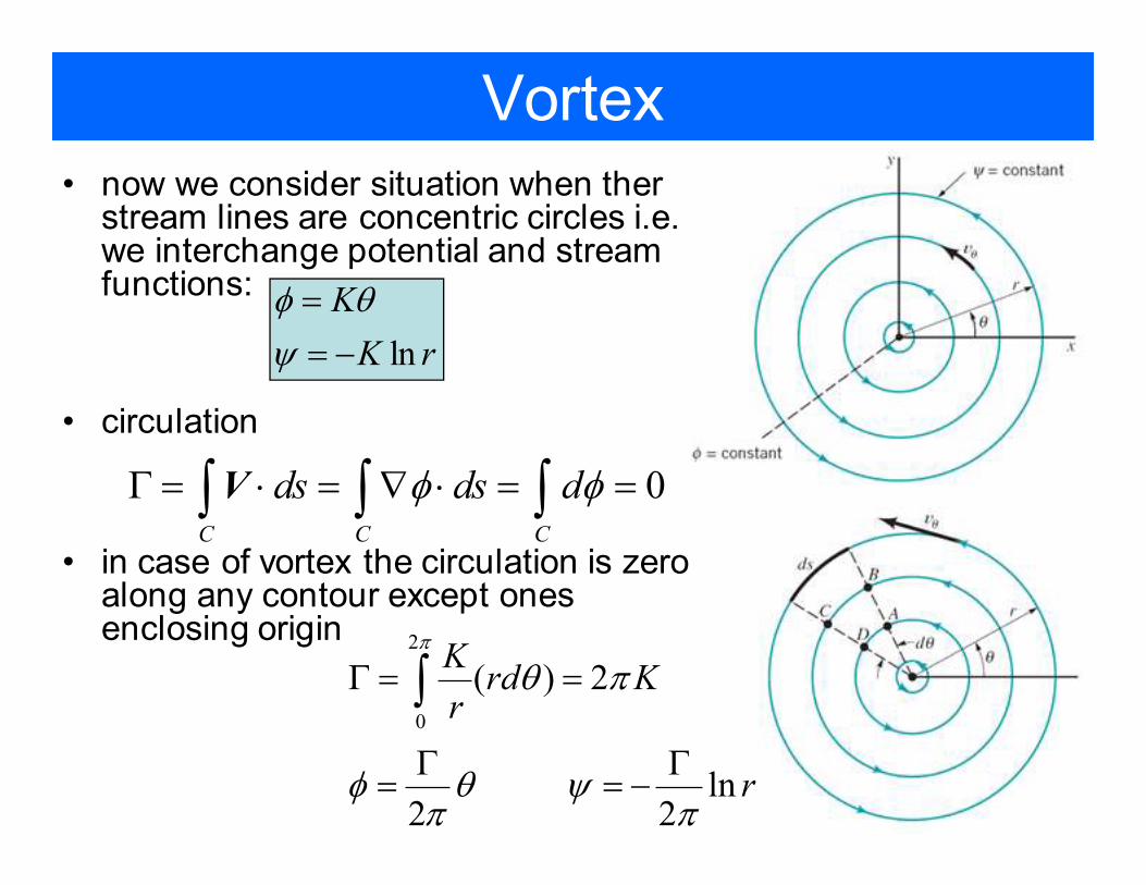
Vortex

• now we consider situation when ther stream lines are concentric circles i.e. we interchange potential and stream functions:

ln

K

K r

φ θ

ψ

=

= −

• circulation

0C C C

ds ds dφ φΓ = ⋅ = ∇ ⋅ = =∫ ∫ ∫� � �V

• in case of vortex the circulation is zero along any contour except ones enclosing origin 2

0

( ) 2

ln2 2

Krd K

r

r

π

θ π

φ θ ψπ π

Γ = =

Γ Γ= = −

∫

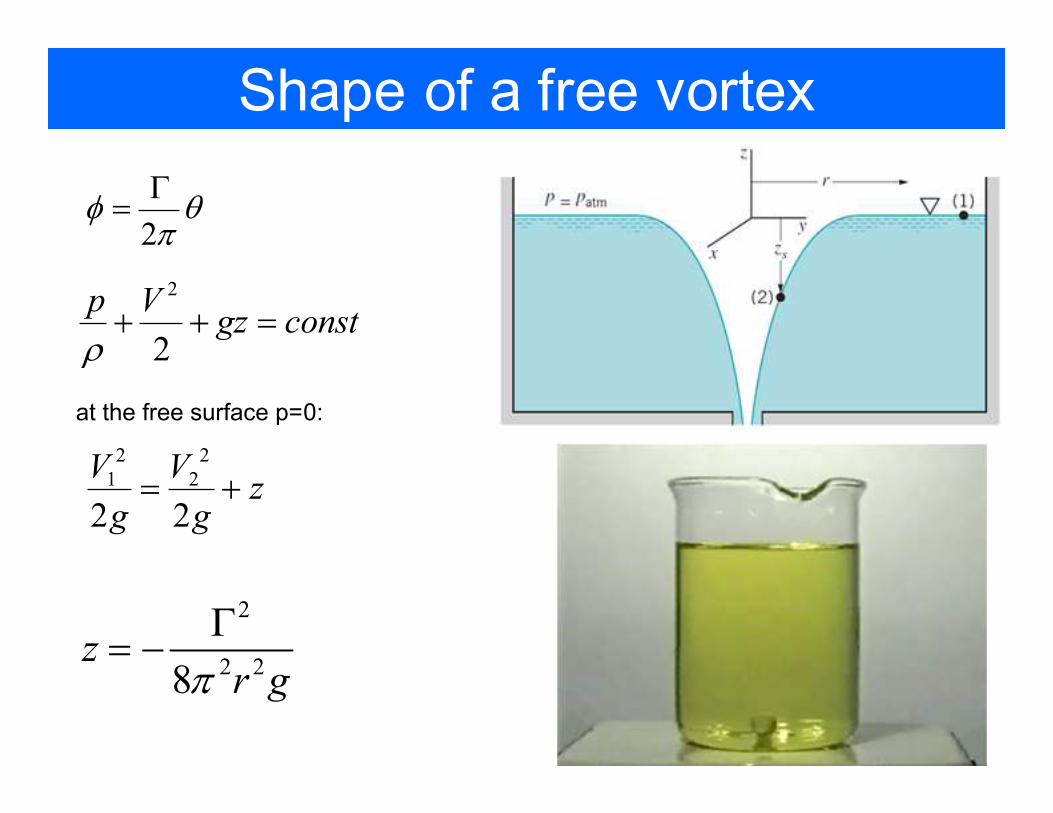
Shape of a free vortex

2φ θ

πΓ

=

2

2

p Vgz const

ρ+ + =

2 2

1 2

2 2

V Vz

g g= +

at the free surface p=0:

2

2 28

zr gπ

Γ= −

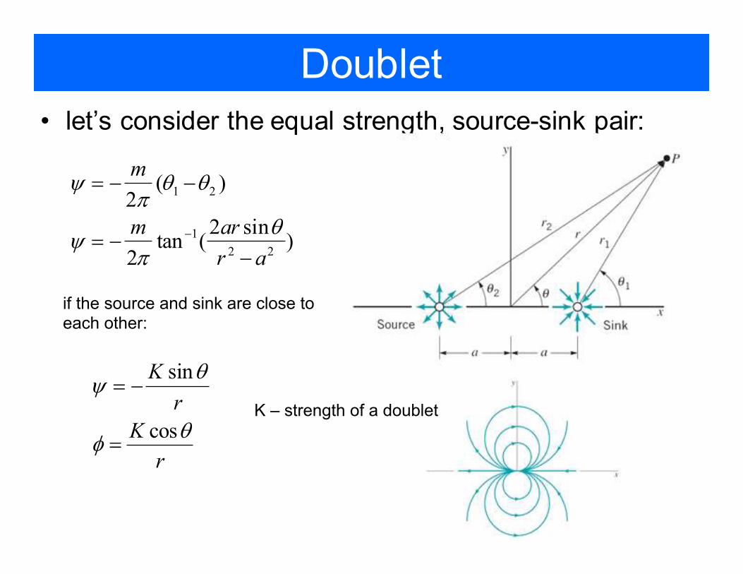
Doublet

• let’s consider the equal strength, source-sink pair:

1 2( )2

mψ θ θ

π= − −

1

2 2

2 sintan ( )

2

m ar

r a

θψ

π−= −

−

if the source and sink are close to each other:

sin

cos

K

r

K

r

θψ

θφ

= −

=

K – strength of a doublet

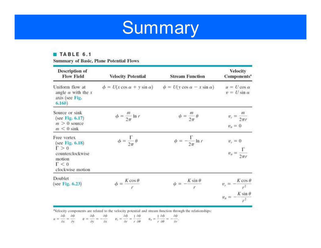
Summary

Superposition of basic flows

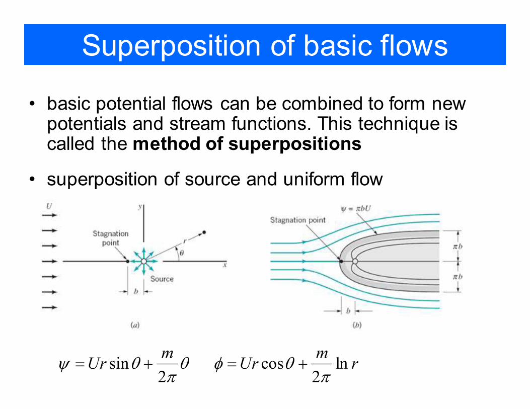
• basic potential flows can be combined to form new potentials and stream functions. This technique is called the method of superpositions

• superposition of source and uniform flow

sin cos ln2 2

m mUr Ur rψ θ θ φ θ

π π= + = +

Superposition of basic flows

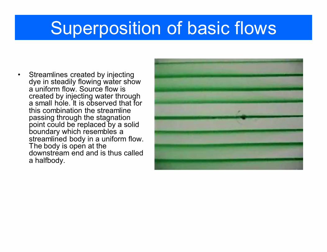
• Streamlines created by injecting dye in steadily flowing water show a uniform flow. Source flow is created by injecting water through a small hole. It is observed that for this combination the streamline passing through the stagnation point could be replaced by a solid boundary which resembles a streamlined body in a uniform flow. The body is open at the downstream end and is thus called a halfbody.

Rankine Ovals

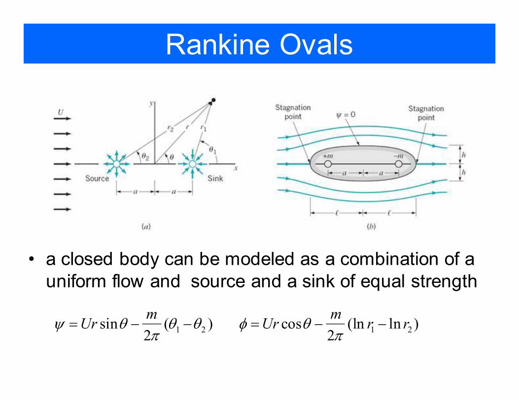
• a closed body can be modeled as a combination of a

uniform flow and source and a sink of equal strength

1 2 1 2sin ( ) cos (ln ln )2 2

m mUr Ur r rψ θ θ θ φ θ

π π= − − = − −

Flow around circular cylinder

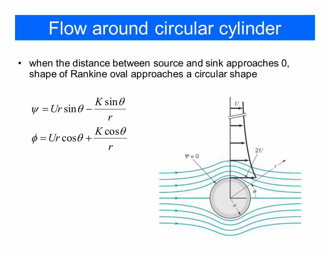
• when the distance between source and sink approaches 0, shape of Rankine oval approaches a circular shape

sinsin

coscos

KUr

r

KUr

r

θψ θ

θφ θ

= −

= +

Potential flows

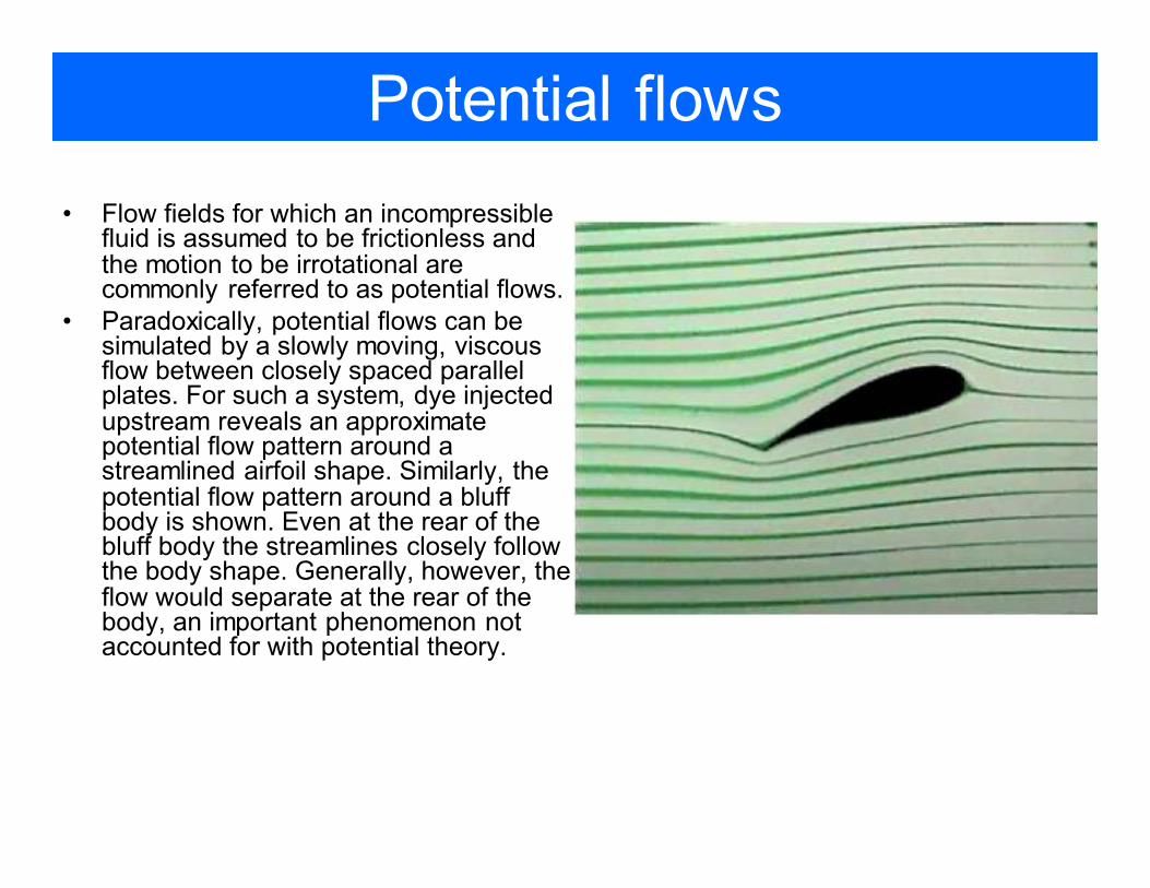
• Flow fields for which an incompressible fluid is assumed to be frictionless and the motion to be irrotational are commonly referred to as potential flows.

• Paradoxically, potential flows can be simulated by a slowly moving, viscous flow between closely spaced parallel plates. For such a system, dye injected upstream reveals an approximate potential flow pattern around a streamlined airfoil shape. Similarly, the potential flow pattern around a bluff body is shown. Even at the rear of the bluff body the streamlines closely follow the body shape. Generally, however, the flow would separate at the rear of the body, an important phenomenon not accounted for with potential theory.

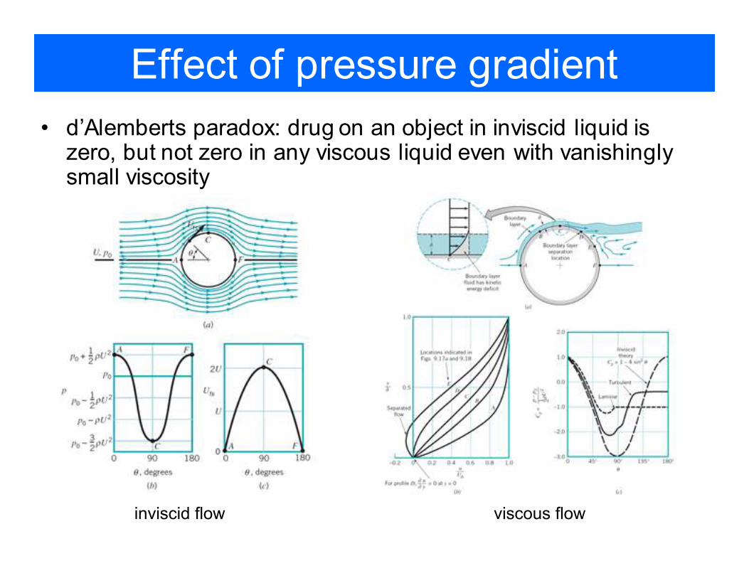
Effect of pressure gradient

• d’Alemberts paradox: drug on an object in inviscid liquid is zero, but not zero in any viscous liquid even with vanishingly small viscosity

inviscid flow viscous flow

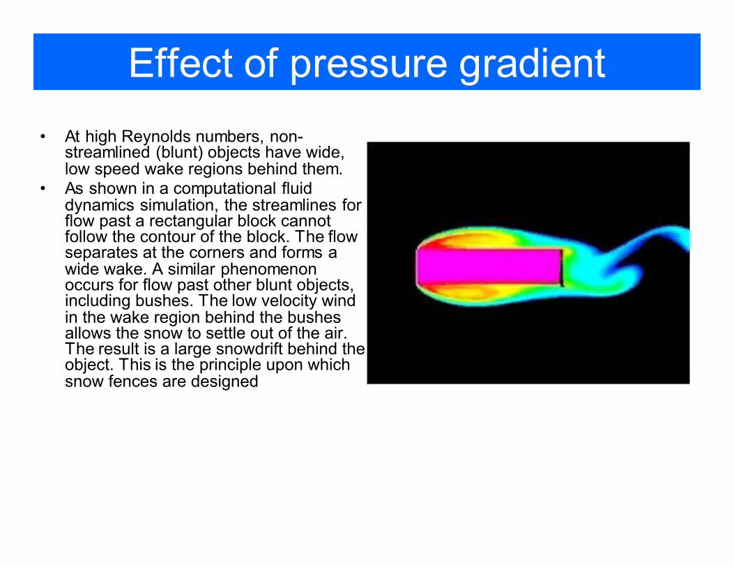
Effect of pressure gradient

• At high Reynolds numbers, non-streamlined (blunt) objects have wide, low speed wake regions behind them.

• As shown in a computational fluid dynamics simulation, the streamlines for flow past a rectangular block cannot follow the contour of the block. The flow separates at the corners and forms a wide wake. A similar phenomenon occurs for flow past other blunt objects, including bushes. The low velocity wind in the wake region behind the bushes allows the snow to settle out of the air. The result is a large snowdrift behind the object. This is the principle upon which snow fences are designed

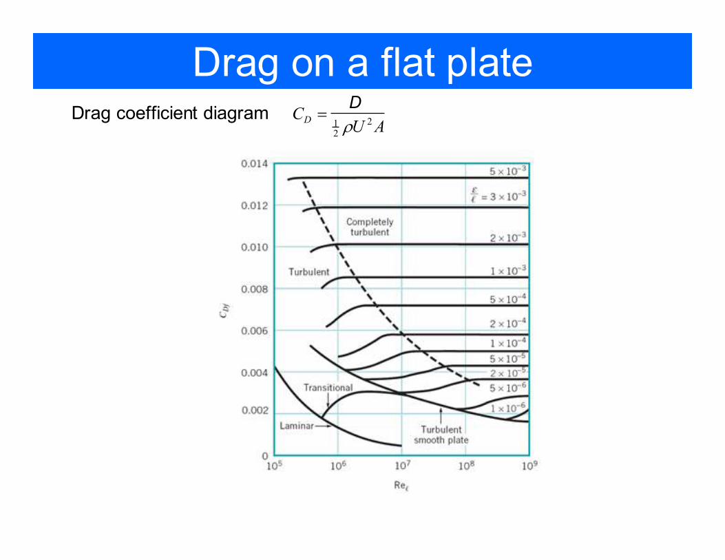
Drag on a flat plateDrag coefficient diagram

212

DCU Aρ

=D

Drag dependence

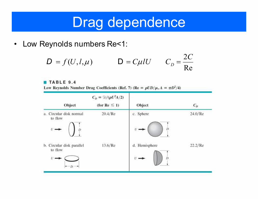
• Low Reynolds numbers Re<1:

2( , , )

ReD

Cf U l C lU Cµ µ= = =D D

Drag dependence

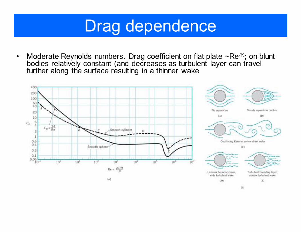
• Moderate Reynolds numbers. Drag coefficient on flat plate ~Re-½; on blunt bodies relatively constant (and decreases as turbulent layer can travel further along the surface resulting in a thinner wake

Examples

Examples

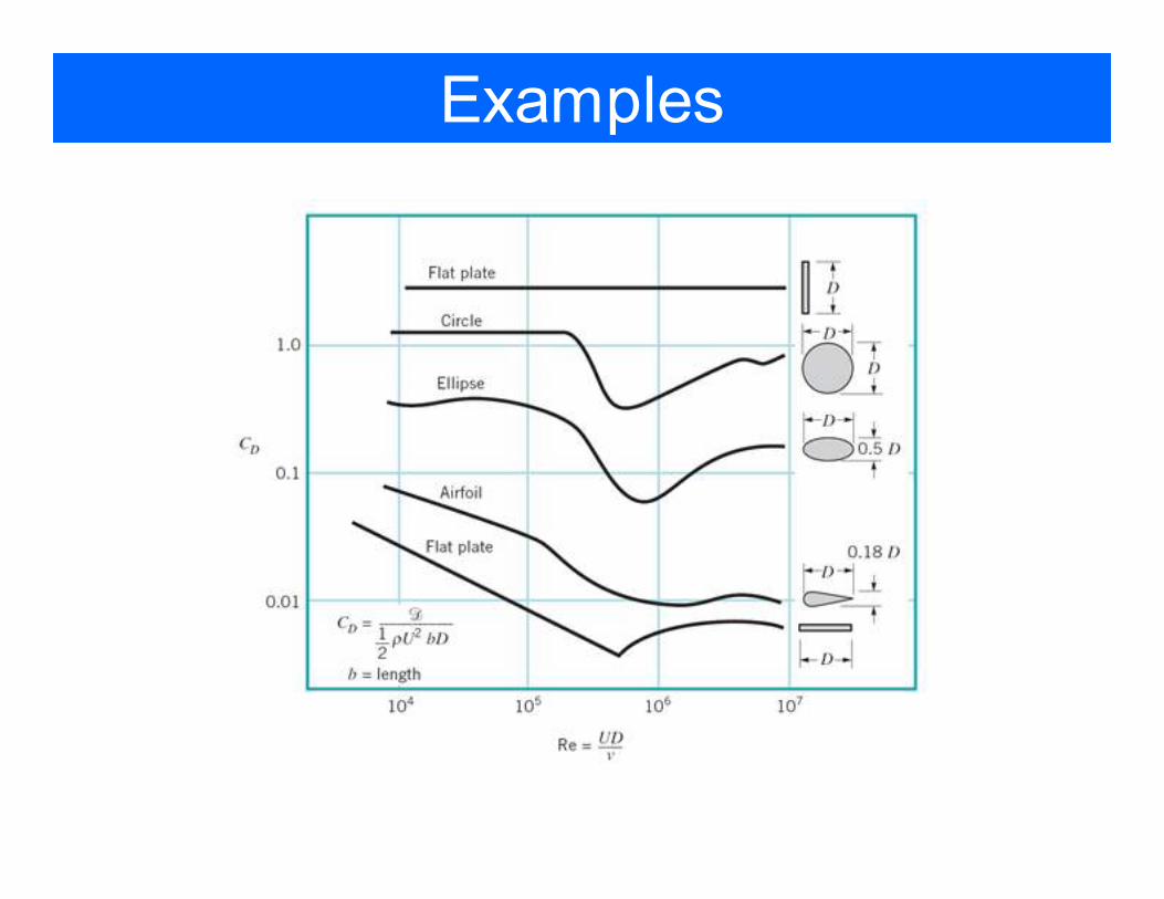
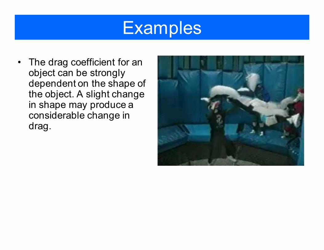
• The drag coefficient for an object can be strongly dependent on the shape of the object. A slight change in shape may produce a considerable change in drag.

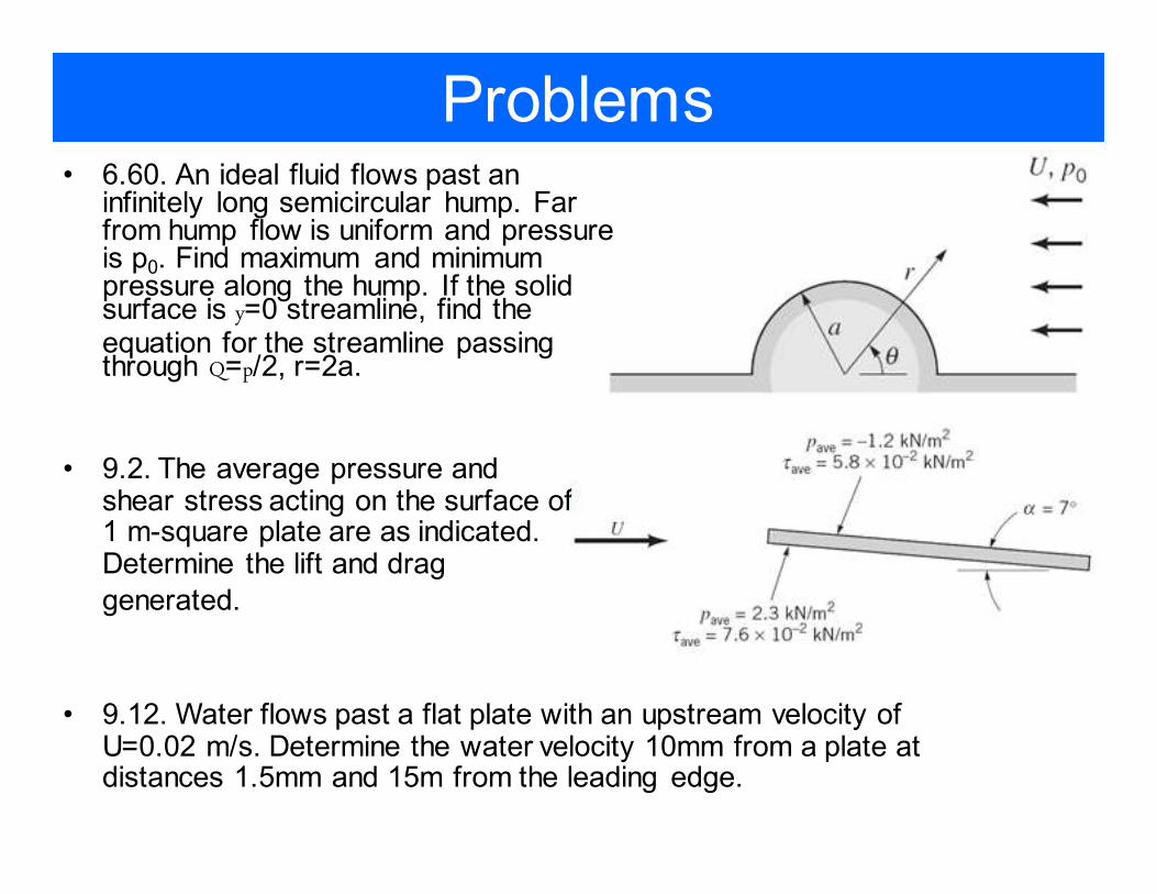
Problems• 6.60. An ideal fluid flows past an

infinitely long semicircular hump. Far from hump flow is uniform and pressure is p0. Find maximum and minimum pressure along the hump. If the solid surface is y=0 streamline, find the equation for the streamline passing through Q=p/2, r=2a.

• 9.2. The average pressure and shear stress acting on the surface of 1 m-square plate are as indicated. Determine the lift and drag

generated.

• 9.12. Water flows past a flat plate with an upstream velocity of U=0.02 m/s. Determine the water velocity 10mm from a plate at distances 1.5mm and 15m from the leading edge.