Lecture 7 Rolling Constraints The most common, and most important nonholonomic constraints They cannot be wri5en in terms of the variables alone you must include some deriva9ves The resul9ng differen9al is not integrable 1
Transcript
Lecture 7 Rolling Constraints
The most common, and most important nonholonomic constraints
They cannot be wri5en in terms of the variables alone you must include some deriva9ves
The resul9ng differen9al is not integrable
1
The major assump9on/simplifica9on is point contact
This is true of a rigid hoop on a rigid surface
or a rigid sphere on a rigid surface
2
I will also generally assume that the surface is horizontal so that gravity is normal to the surface
3
rigid hoop on a rigid surface
4
rigid sphere on a rigid surface
5
It’s not a bad approxima9on for a well‐inflated bicycle or motorcycle 9re on hard pavement
It’s not so good for an automobile 9re, which has a pre5y big patch on the ground
Cylindrical wheels, like those on grocery carts and children’s toys must slip over parts of their surfaces when turning
We aren’t going to care about any of this We’re going to suppose that all the wheels we consider have point contact
6
Two fundamental ideas:
The speed of a point rota9ng about a fixed point is
€
v =ω × r
The contact point between a wheel and the ground is not moving
We can view the 9me deriva9ve of q as a surrogate for δq
€
C jiδq j = 0
€
dI η( )dη
= 0 =∂L *∂qk −
ddt
∂L *∂ ˙ q k
∂qk
∂ηdt
t1
t2∫ =∂L *∂qk −
ddt
∂L *∂ ˙ q k
δqkdt
t1
t2∫
Now let’s go back to lecture two and the ac9on integral it is sta9onary if
Consider the final version
14
€
∂L *∂qk −
ddt
∂L *∂ ˙ q k
δqkdt
t1
t2∫ = 0
and let’s add mul9ples of the constraints to this They are zero, so there’s no problem
€
∂L *∂qk −
ddt
∂L *∂ ˙ q k
δqkdt
t1
t2∫ = 0
€
λiC jiδq j = 0
€
λiCkiδqk = 0
mul9ply each row by its own constant
change the dummy index j to k
15
€
∂L *∂qk −
ddt
∂L *∂ ˙ q k
+ λiCk
i
δqkdt
t1
t2∫ = 0
drop the asterisk and incorporate external forces directly the constrained Euler Lagrange equa9ons
€
ddt
∂L∂ ˙ q k
−
∂L∂qk = λiCk
i + Qk
I have added as many variables as there are nonholonomic constraints
I need as many extra equa9ons, which are the constraints themselves
16
€
ddt
∂L∂ ˙ q k
−
∂L∂qk = λiCk
i + Qk
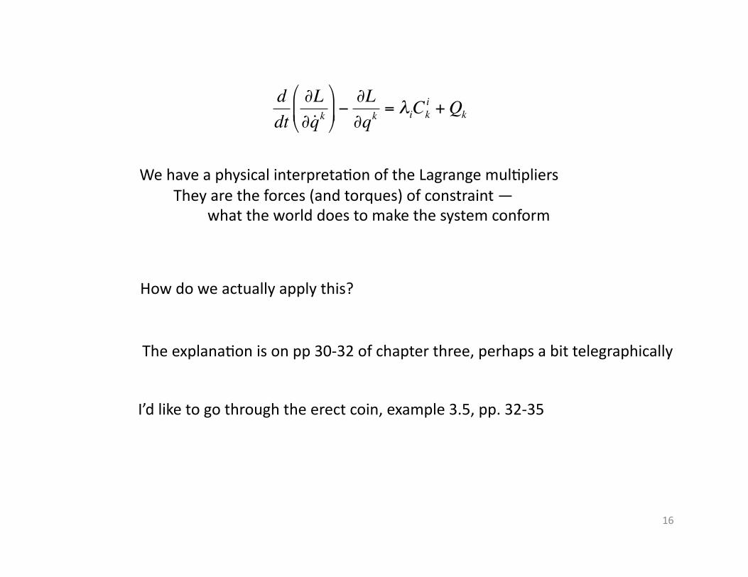
We have a physical interpreta9on of the Lagrange mul9pliers They are the forces (and torques) of constraint — what the world does to make the system conform
How do we actually apply this?
The explana9on is on pp 30‐32 of chapter three, perhaps a bit telegraphically
I’d like to go through the erect coin, example 3.5, pp. 32‐35
17
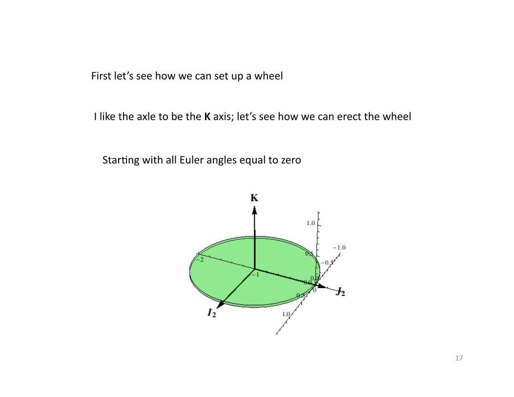
First let’s see how we can set up a wheel
I like the axle to be the K axis; let’s see how we can erect the wheel
Star9ng with all Euler angles equal to zero
18
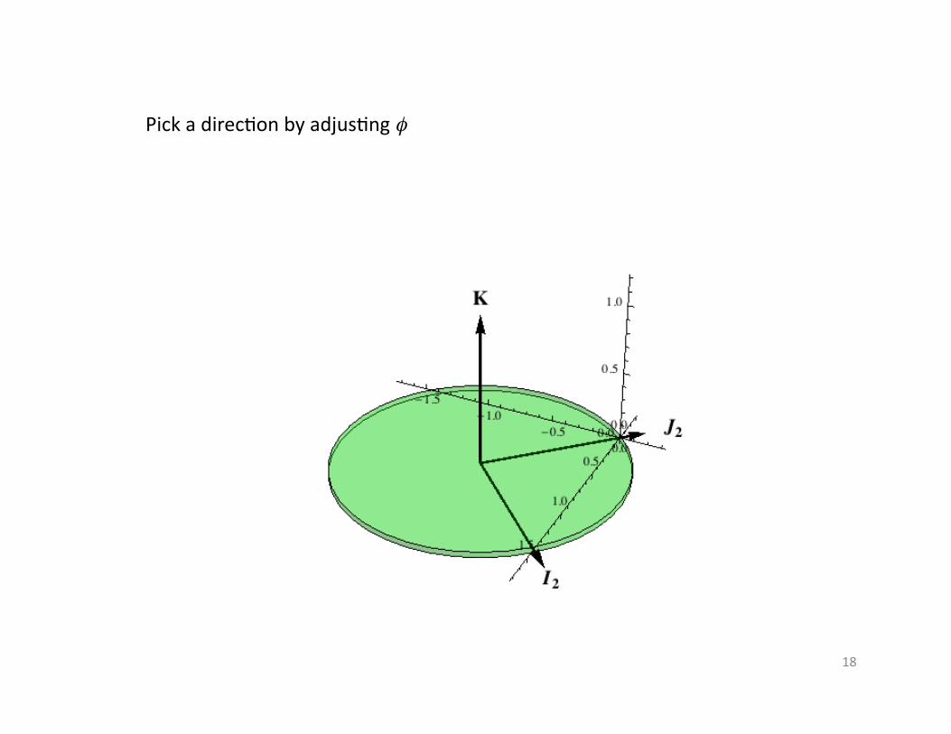
Pick a direc9on by adjus9ng φ
19
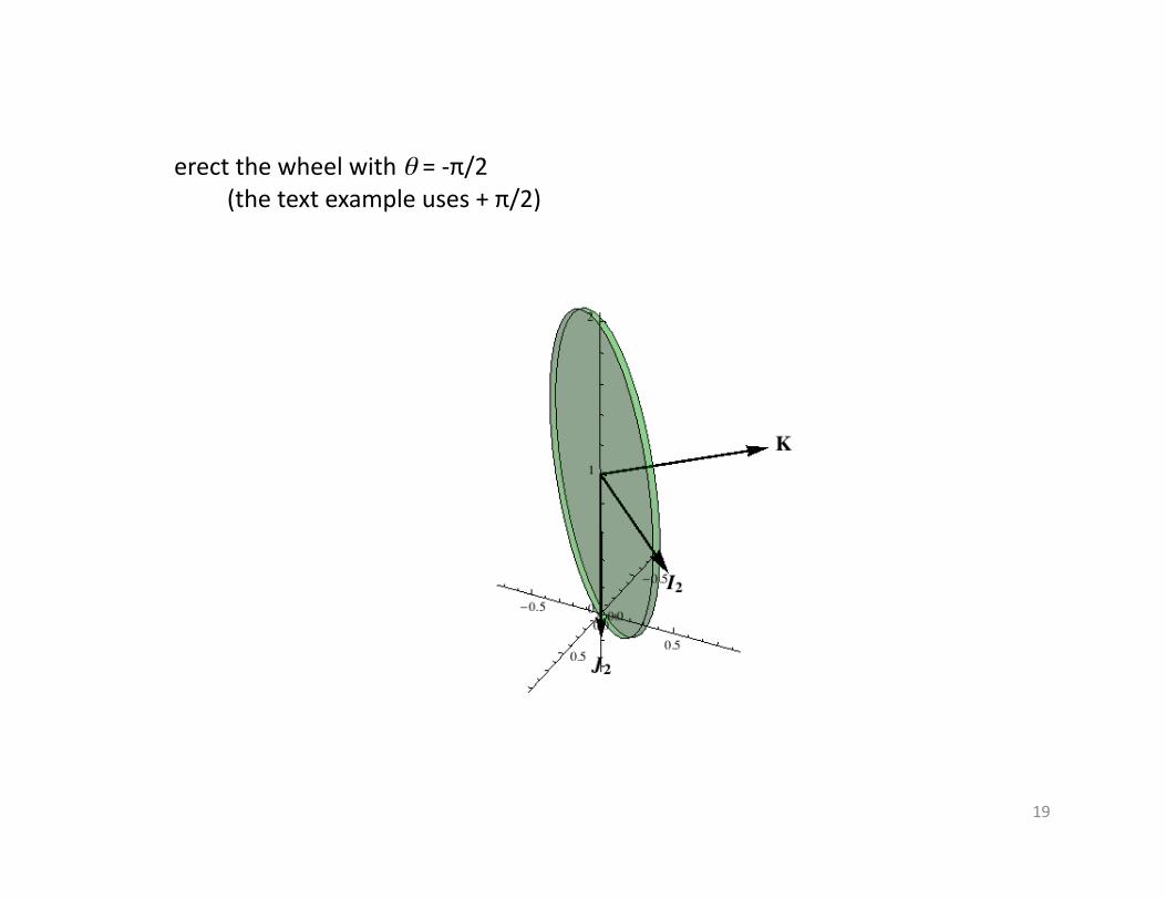
erect the wheel with θ = ‐π/2 (the text example uses + π/2)
20
€
r = −aJ2, ω = ˙ ψ K
€
v =ω × r = − ˙ ψ K × aJ2 = a ˙ ψ I2 = a ˙ ψ
cosφsinφ
0
€
˙ x − a ˙ ψ cosφ = 0 = ˙ y − a ˙ ψ sinφ
Variables are x, y, φ and ψ — z and θ are fixed
ω has a k component, but it’s perpendicular to r
21
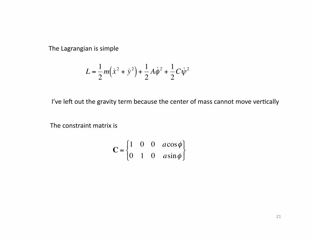
The Lagrangian is simple
€
L =12
m ˙ x 2 + ˙ y 2( ) +12
A ˙ φ 2 +12
C ˙ ψ 2
I’ve lek out the gravity term because the center of mass cannot move ver9cally
The constraint matrix is
€
C =1 0 0 acosφ0 1 0 asinφ
22
The product
€
λC = λ1 λ2{ }1 0 0 acosφ0 1 0 asinφ
= λ1 λ2 0 a λ1 cosφ + λ2 sinφ( ){ }
The Lagrange equa9ons are then
€
m˙ ̇ x = λ1, m˙ ̇ y = λ2, ˙ ̇ φ = 0, ˙ ̇ ψ =aC
λ1 cosφ + λ2 sinφ( )
and the constraints are
€
˙ x − a ˙ ψ cosφ = 0 = ˙ y − a ˙ ψ sinφ
23
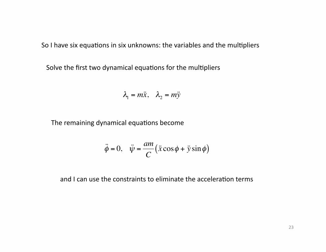
So I have six equa9ons in six unknowns: the variables and the mul9pliers
Solve the first two dynamical equa9ons for the mul9pliers
€
λ1 = m˙ ̇ x , λ2 = m˙ ̇ y
The remaining dynamical equa9ons become
€
˙ ̇ φ = 0, ˙ ̇ ψ =amC
˙ ̇ x cosφ + ˙ ̇ y sinφ( )
and I can use the constraints to eliminate the accelera9on terms
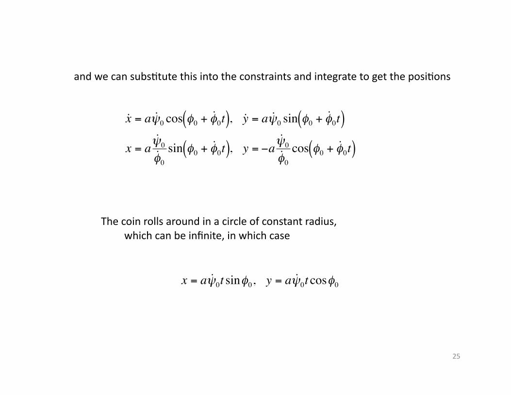
24
€
˙ x − a ˙ ψ cosφ = 0 = ˙ y − a ˙ ψ sinφ⇓
˙ ̇ x = a ˙ ̇ ψ cosφ − a ˙ ψ ̇ φ sinφ, ˙ ̇ y = a ˙ ̇ ψ sinφ + a ˙ ψ ̇ φ cosφ