Contents:

Textbook:

Example:

Topic 7

Two- and Three­Dimensional SolidElements; PlaneStress, PlaneStrain, andAxisymmetricConditions

• Isoparametric interpolations of coordinates anddisplacements

• Consistency between coordinate and displacementinterpolations

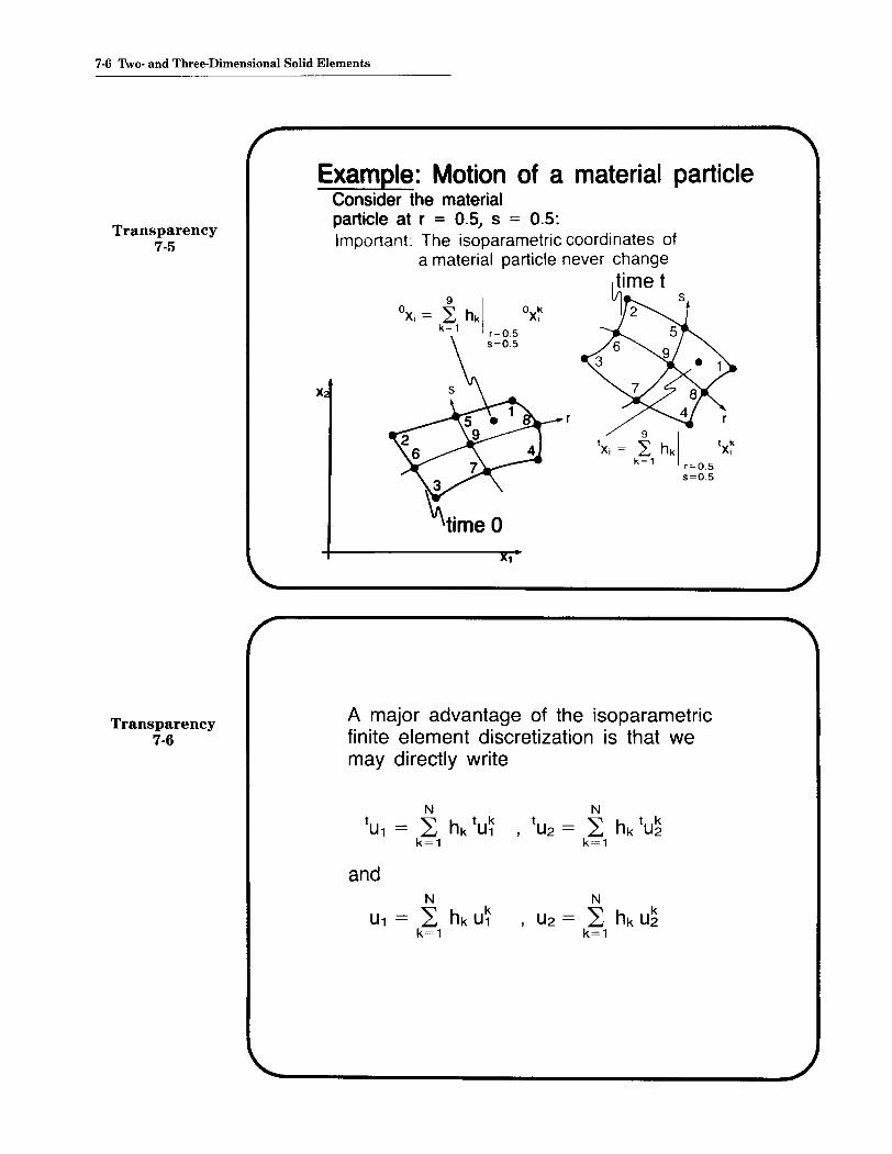
• Meaning of these interpolations in large displacementanalysis, motion of a material particle

• Evaluation of required derivatives

• The Jacobian transformations

• Details of strain-displacement matrices for total andupdated Lagrangian formulations

• Example of 4-node two-dimensional element, details ofmatrices used

Sections 6.3.2, 6.3.3

6.17

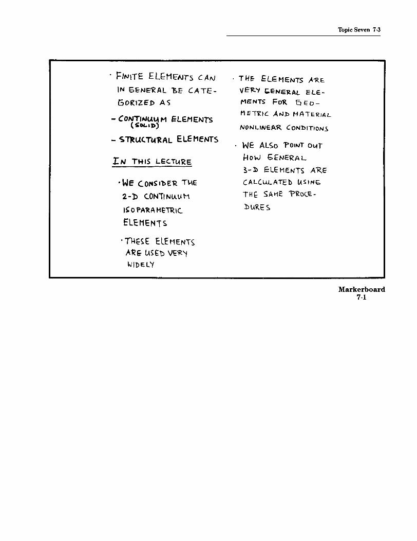
• J=INITE ELfHEAlrs CAN

IN 5ENE'KAl ~E CATE­

GORIZE]) AS

- CONTINlA~ M ELE.MENTs( ~oc..'J»

- S~U(TLfRAL ELEMENTS

I.N THIS LEC.TlARE

•We CONSlbE'R T\-\E

2-b C.ON'I NlA,U M

I~ 0 PA'RA HETT<\C.

ELEMENTS.

. TI4~~E ELf HE:NT~ARE- US~'t> VE'1C'IWIDE.l'(

T 11E- ElE MENTS .A'RE.

VE~~ ~ENe~AL ELE­MENTS FoR Q ~o-

MET~IC ANb H ATJ;R.AL

NONLINEAR. CONl:>ITIONS

WE Al<;o 'POINT O\AT

How bfNERAL

5-]) ElEHENTS ARE

CALClALATEb (As INb

TH I: SA~E '?~O(E-

)) U~E S.

Topic Seven 7-3

Markerboard7-1

7-4 Two- and Three-Dimensional Solid Elements

Transparency7-1

Transparency7-2

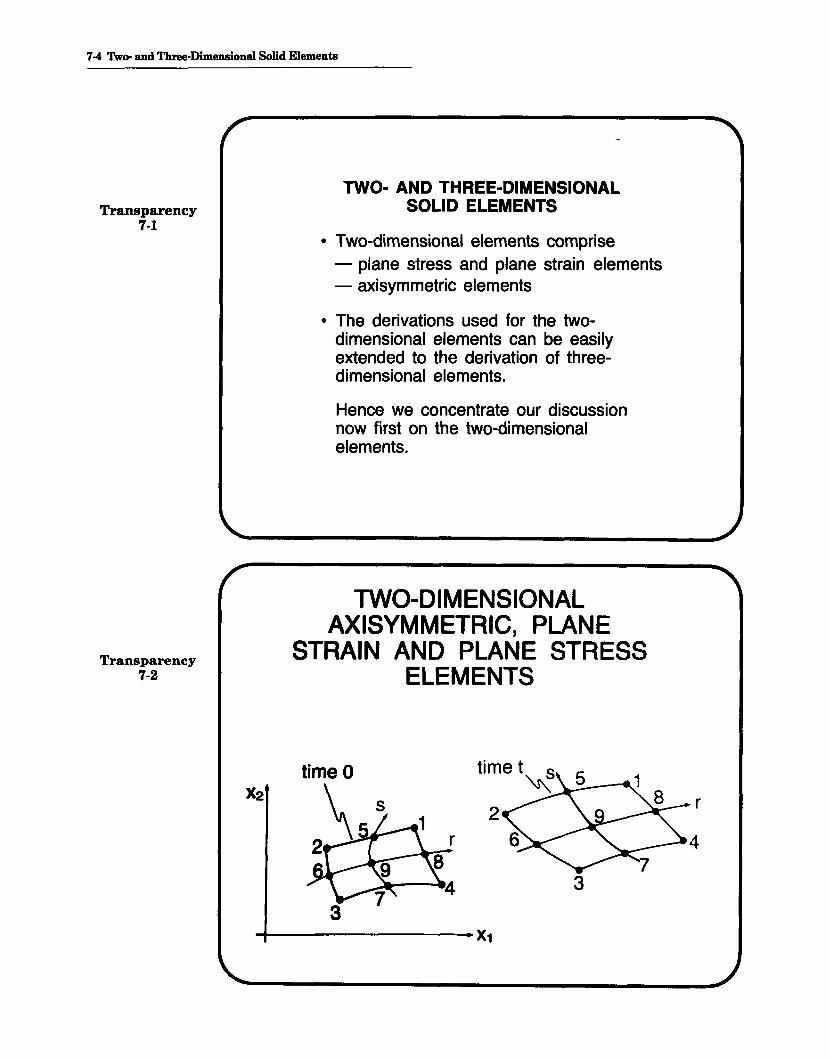
TWO- AND THREE-DIMENSIONALSOLID ELEMENTS

• Two-dimensional elements comprise- plane stress and plane strain elements- axisymmetric elements

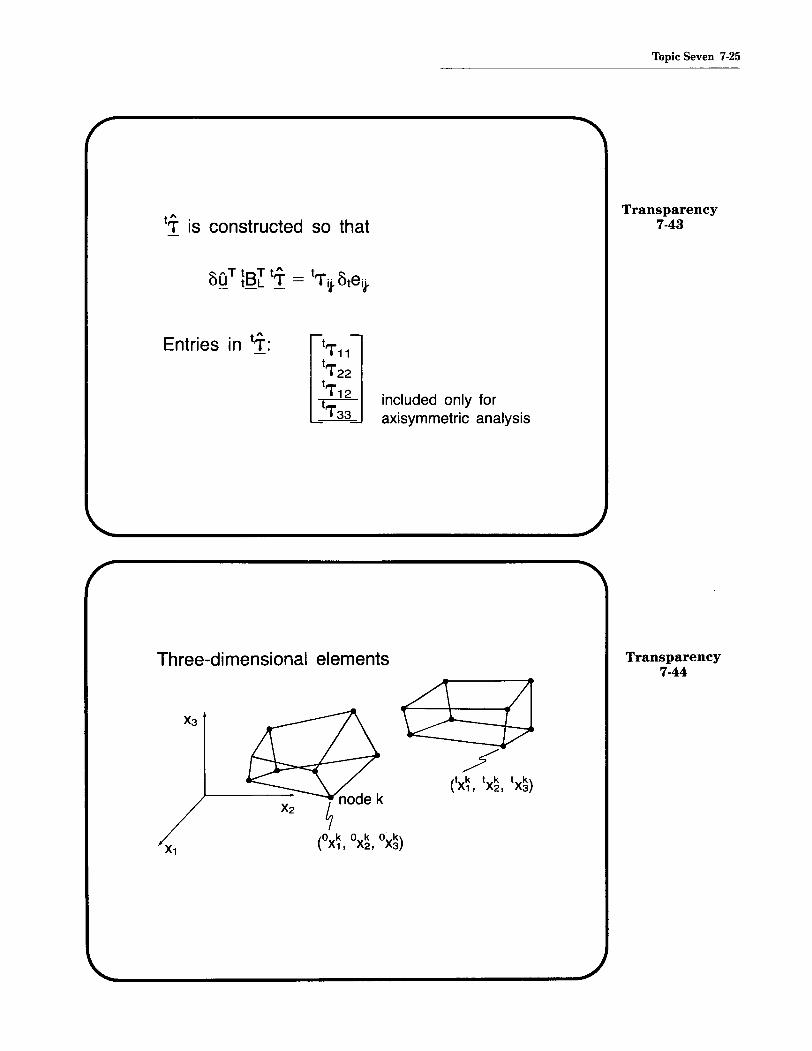
• The derivations used for the two­dimensional elements can be easilyextended to the derivation of three­dimensional elements.

Hence we concentrate our discussionnow first on the two-dimensionalelements.

TWO-DIMENSIONALAXISYMMETRIC, PLANE

STRAIN AND PLANE STRESSELEMENTS

3

+----------X1

Topic Seven 7-5

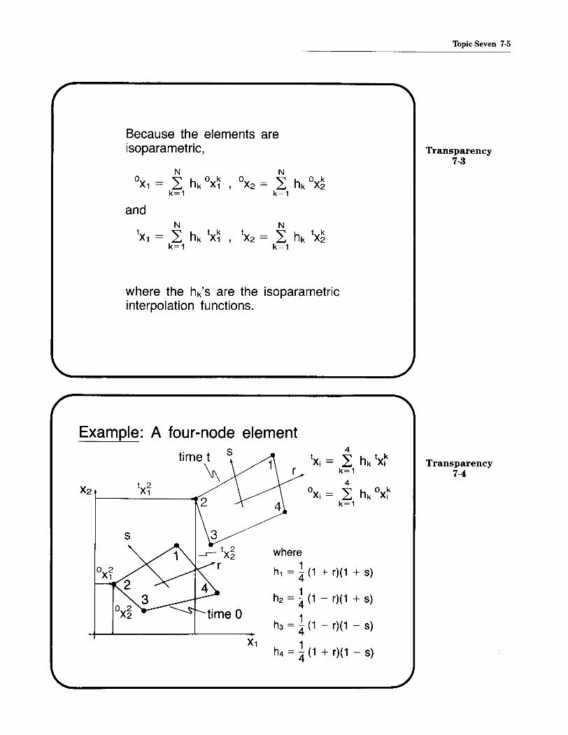
Because the elements areisoparametric, Transparency

7-3N N

0 L hk °x~ ° L hk °x~X1 = , X2 =k=1 k=1

andN Nt L hk tx~ t L hk tx~X1 = , X2 =

k=1 k=1

where the hk's are the isoparametricinterpolation functions.

Transparency7-4

4

tXi = L hk tx~k=1

4

°Xi = 2: hk °x~k=1

where1

h1 = 4: (1 + r)(1 + s)

1h2 = - (1 - r)(1 + s)

41

h3 = - (1 - r)(1 - s)41

h4 = 4 (1 + r)(1 - s)

time 0

Example: A four-node elements

7-6 1\vo- and Three-Dimensional Solid Elements

Transparency7-5

r

tx; = t hkl tx~k-1 r;0.5

5=0.5

x

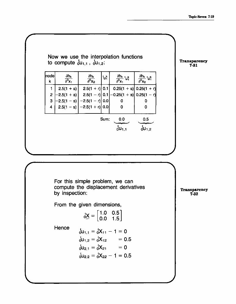
Transparency A major advantage of the isoparametric7-6 finite element discretization is that we

may directly write

N NtU1 ~ hk tu~ t

~ hk tu~U2 =k=1 k=1

andN N

U1 ~ hk u~ U2 = ~ hk u~k=1 k=1

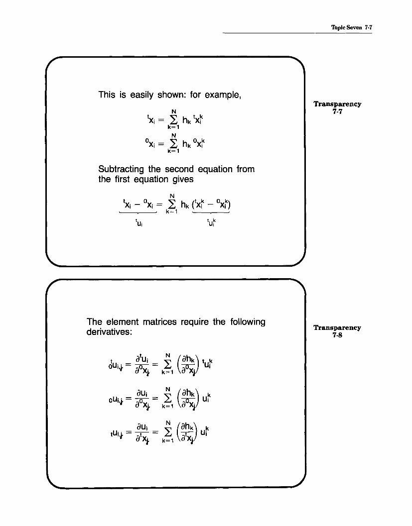
This is easily shown: for example,

Nt ~ h t kXi = £J k Xi

k=1

No ~ h 0 kXi = £J k Xi

k=1

Subtracting the second equation fromthe first equation gives

Nt 0 ~ h (t k 0 k)Xi - Xi = £J k Xi - Xi

, . k=1 ' , .

The element matrices require the followingderivatives:

Topic Seven 7-7

Transparency7-7

Transparency7-8

7-8 'I\vo- and Three-Dimensional Solid Elements

Transparency7·9

Transparency7-10

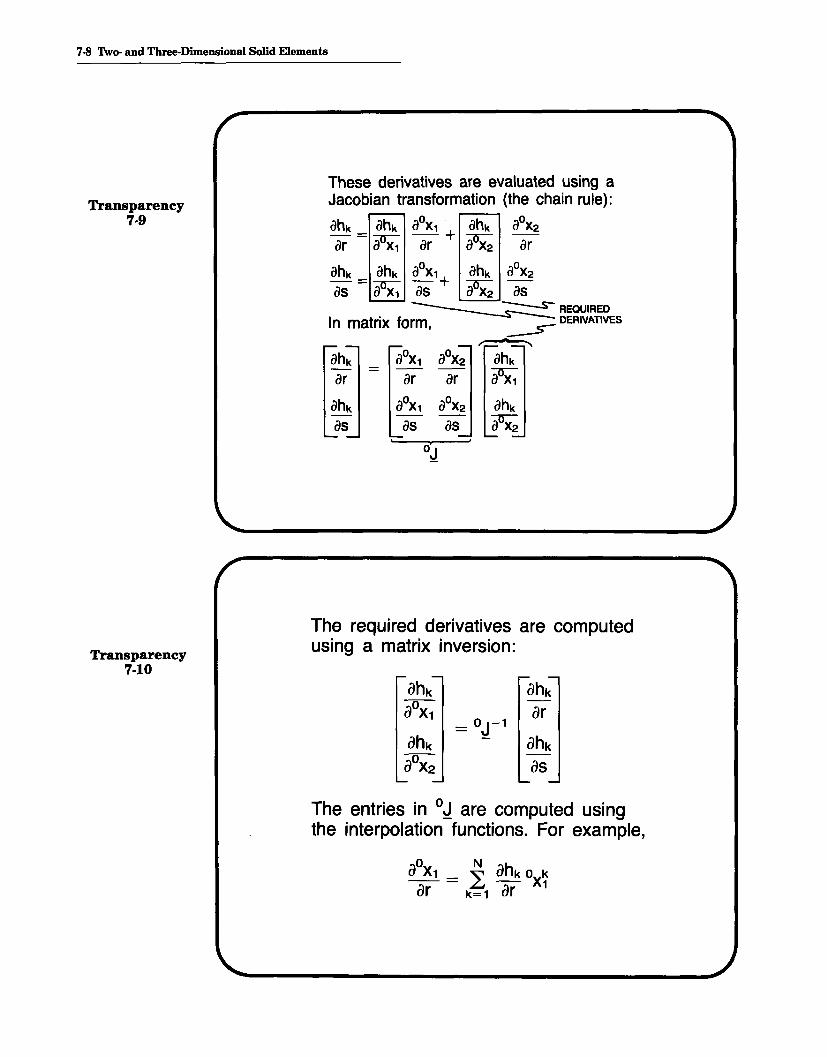
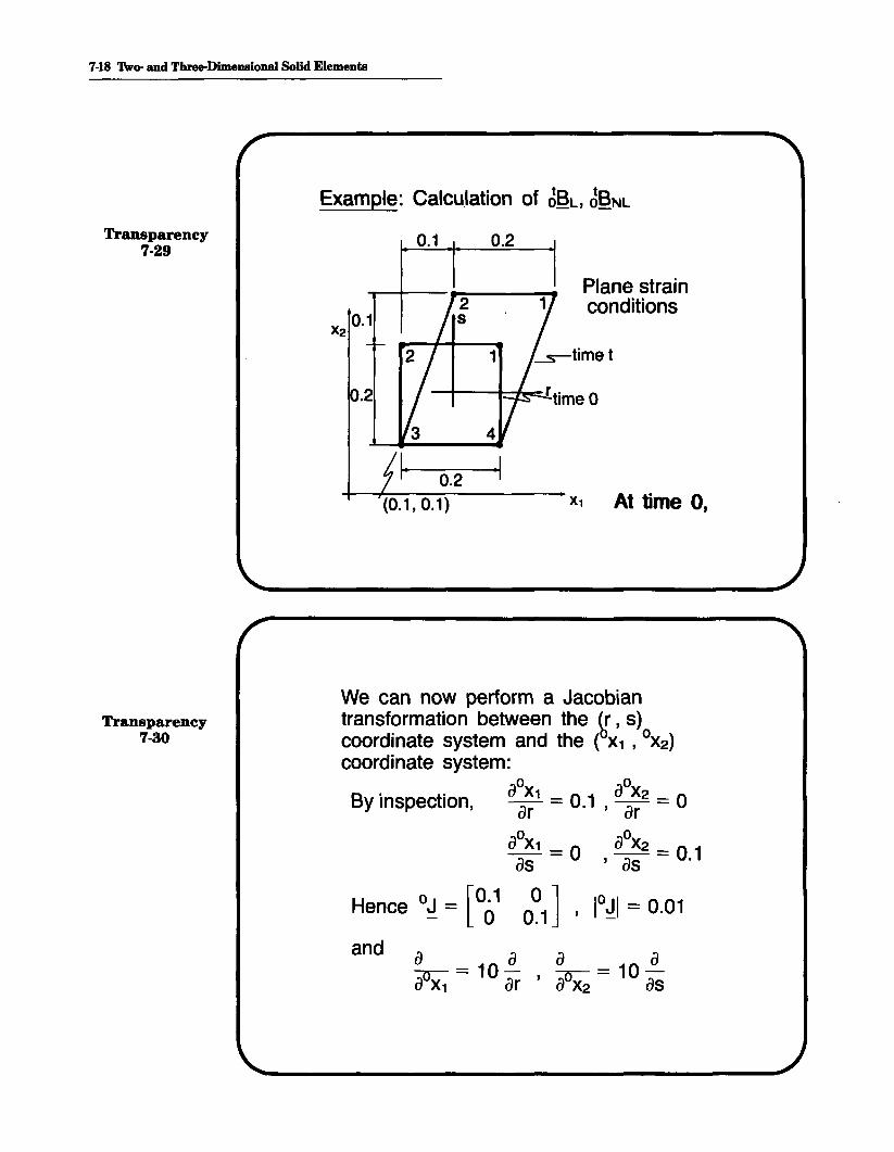
These derivatives are evaluated using aJacobian transformation (the chain rule):

ahk _ ahk aOx1 + ahk aOx2ar - aOx1 ar aOx2 ar

ahk ahk aOx1 ahk aOx2as - aOx1 as + aox;. as

~REaUIREDIn matrix form, ~ DERIVATIVES

r A ,

ahk ilxl aOx2 ahkas as as aOX2

°4

The required derivatives are computedusing a matrix inversion:

ahk ahkaOx1

-

= 0J-1ar

ahk ahkaOx2

-as

The entries in oJ are computed usingthe interpolation functions. For example,

° N ha X1 = L a k 0x~ar k=1 ar

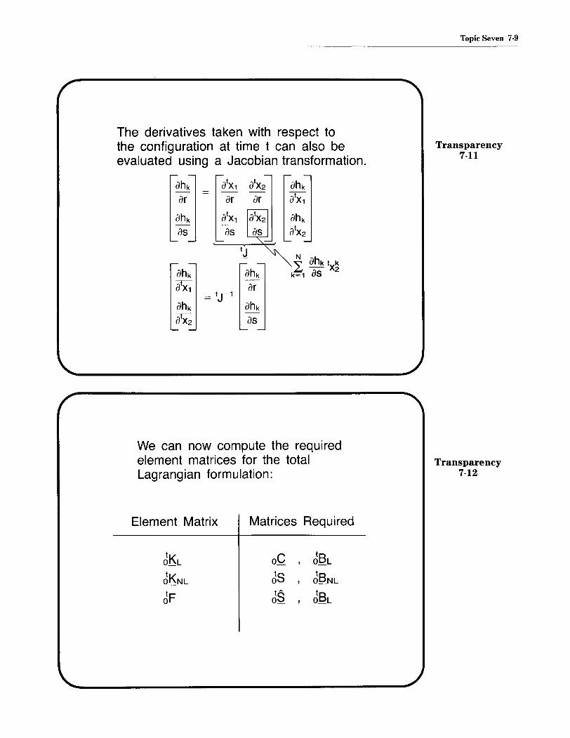
The derivatives taken with respect tothe configuration at time t can also beevaluated using a Jacobian transformation.

ahk a1x1 alX2 ahk- = - -

alX1ar ar ar

ahk a1x1 a1x2 ahk- - -

a1x2as as as

IJ

f ahk IX~ahk ahk k=1 asa1x1

-ar

ahk

= IJ-1ahk

alX2-

as

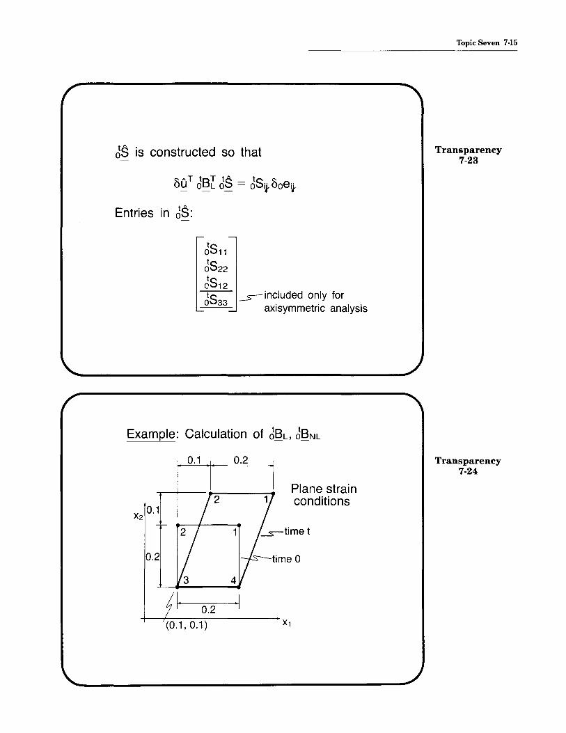
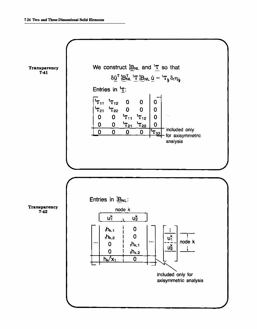
We can now compute the requiredelement matrices for the totalLagrangian formulation:

Topic Seven 7-9

Transparency7-11

Transparency7-12

Element Matrix Matrices Required

oC , dBL

ds , dBNLtAtoS , oBL

7-10 Two- and Three-Dimensional Solid Elements

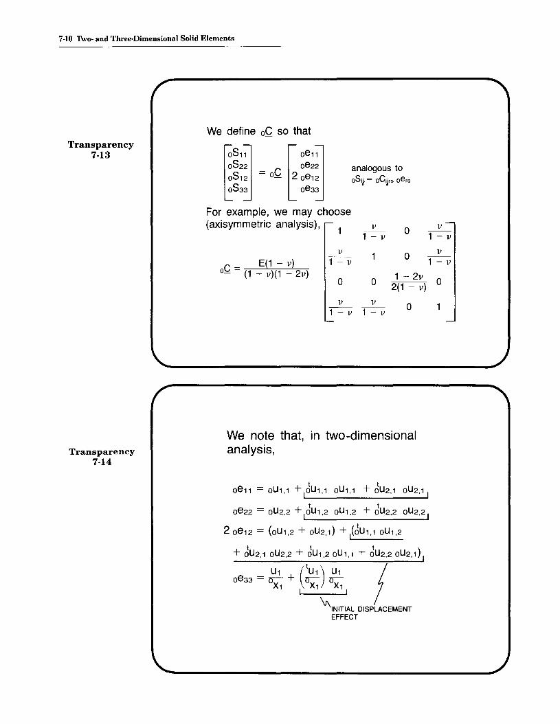
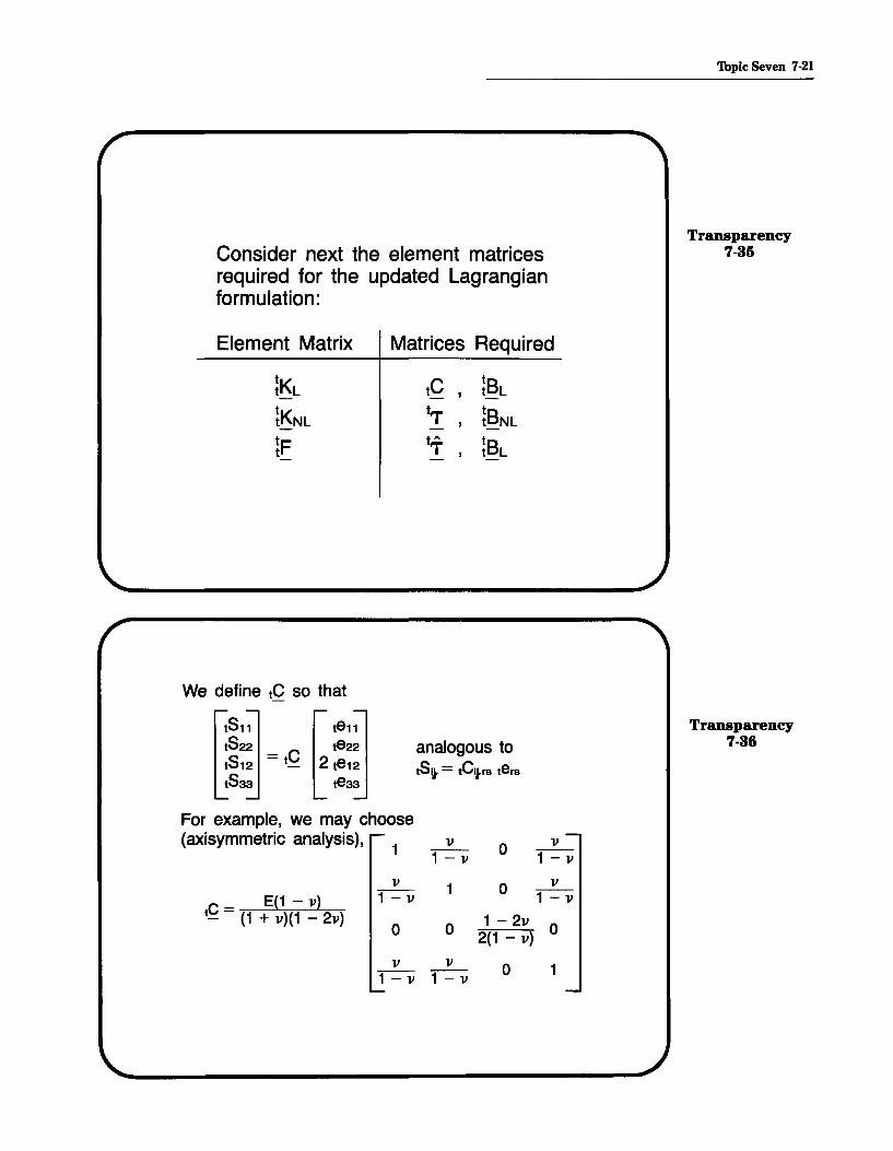
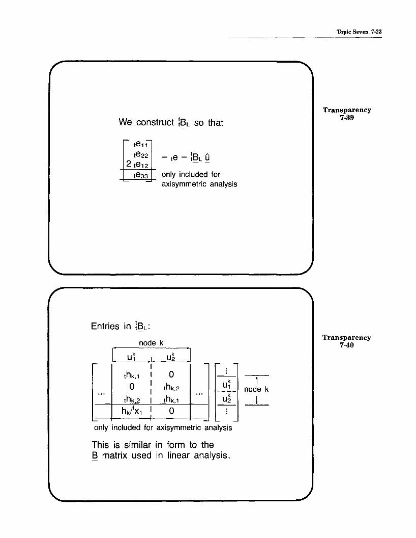
We define oC so thatTransparency

7-13 0811

0822

0812

0833

analogous toOSij. = oC~,s oe,s

1

For example, we may choose(axisymmetric analysis), v

1 - v o

Transparency7-14

v 0v

_ E(1 - v) 1 - v 1 - voQ - (1 + v)(1 - 2v)

0 01 - 2v

02(1 - v)

v v 01 - v 1 - v

We note that, in two-dimensionalanalysis,

t tOe11 = OU1,1 +loU1,1 OU1,1 + OU2,1 OU2,1,

t tOe22 = OU2,2 + IOU 1,2 oU 1,2 + OU2,2 OU2,2,

2 Oe12 = (OU1,2 + OU2,1) + ,(JU 1,1 OU1,2

t t t )

~e:~: ;~2: +(~~~1)2O:~" +°fU2

,2 OU2,1 IX1 X1 X1

I I

""-INITIAL DISPLACEMENTEFFECT

and

1 (U1)201")33 = 2 Ox1

Derivation of 0833, o~:

X2 ./' time 0 /time t+dt

axis of r-\ CIreVolut~ L-:=1 ~

'"---------- X1

We see that

Topic Seven 7-11

Transparency7-15

Transparenc)7-16

7-12 'I\vo- and Three-Dimensional Solid Elements

Transparency7-17

Hence H.1t _1 [(H.1tdS)2 ]oE33 - - ----0-:;-:- - 1

2 ds

Transparency7-18

We construct riBl so that

~oe11]Oe22 t t

2 Oe12 = o~ = (06l0 + 06L1) aDe.. I ~

J JBL

contains initialOe33 is only included displacement effect

for axisymmetric analysis

'Ibpic Seven 7-13

Entries in 6Sl0:node k

..... . . . . -Iohk,1 I 0

0 I ohk,2... ...ohk,2

Iohk,1I

hkfx1 I 0I- -

u~

u~

tnode k

l

Transparency7-19

included only foraxisymmetric analysis

This is similar in form to the B matrix used inlinear analysis.

Transparency7-20u~

node k

- .. . -6U1,1 ohk,1 I 6U2,1 ohk,1

I6U1,20hk,2 I 6U2,20hk,2... I ...6U1,1 Ohk,2 I 6U2,10hk,2

t h I + 6U2,2 ohk,1+ OU1,2 0 k,1 ItU1 hk I

°X1 °X1I 0I

~ I -

Entries in 6Bl1:

I u~

Th ... I d' I t ff t included onlye Inltla ISP acemen e ec tu for axisym~etric

is contained in the terms 6Ui,~, OX:. analysIs

7-14 1\vo- and Three-Dimensional Solid Elements

Transparency7-21

We construct dSNL and ds so that

s:: ~ T tST ts ts ~ ts s::u!! O_NL 0_ O_NL!! = ° i}Uolli}

Entries in ds:

r- -dS11 dS12 0 0 0dS21 dS22 0 0 0

0 0 dS11 dS12 00 0 dS21 dS22 00 0 0 0 dS33..... - included only

for axisymmetricanalysis

Transparency7-22

Entries in dSNL:

node k

u~ ,I u~

tnode k

1

u~---u~

r- I -ohk,1 I 0ohk,2 I 0

I... 0 I Ohk1 ...0 I ohk,2I

hk/OX1 I 0L- I -f

included only foraxisymmetricanalysis

t A

oS is constructed so that

Entries in JS:

Topic Seven 7-15

Transparency7-23

JS11J822

J812

J833~ included only for

axisymmetric analysis

7-16 'I\vo- and Three-Dimensional Solid Elements

Exam~: Calculation of JBlI JBNl

Transparency7-25

0.1 0.2

X2 0.1

0.2

Plane strainconditions

t-+ -l-.L"'"--time 0

Exam~: Calculation of JBlI JBNl

Transparency7-26

0.1 0.2

Plane strainconditions

·1

4

2

0.2

r-t:======:i.J-J-....~time 0material fibershave only translatedrigidly

.2

X2 0.1

(0.1,0.1 )

Example: Calculation of dBL • dBNL

Topic Seven 7-17

0.2

0.1

0.2(0.1,0.1)

0.2

Plane strainconditions

x,

Transparency7-27

Exam~: Calculation of dBLl dBNL

X2 0.1

0.2

0.1

0.2(0.1,0.1)

0.2

·1

Plane strainconditions

time 0material fibers havestretched and rotated

x,

Transparency7-28

7-18 Two- and Three-Dimensional Solid Elements

Transparency7-29

Exam~: Calculation of JBL, JBNL

0.1 0.2

At time 0,

·1

1

Plane strain2 condffionss

0.2

---1----t~~rtime 0

(0.1.0.1)

0.2

X2 0.1

By inspection,

Hence oJ = [0.1- °and a a a a

:;CC-a = 1°-a ':;CC-a = 1°-aX1 r X2 s

We can now perform a Jacobiantransformation between the [, s)coordinate system and the ( X1 ,OX2)

coordinate system:

° °a x1 = °1 a X2 = °ar ., ar

aOx1 = ° aOx2as 'as = 0.1

0~1] , 1°41 = 0.01

Transparency7-30

Now we use the interpolation functionsto compute JU1,1 , JU1,2:

node ahk ahk tu~ ahk t k ahk t kaOx1 aOx2 r U1 - U1

k X1 aOx2

1 2.5(1 + 5) 2.5(1 + r) 0.1 0.25(1 + 5) 0.25(1 + r)

2 -2.5(1 + 5) 2.5(1 - r) 0.1 -0.25(1 + 5) 0.25(1 - r\

3 -2.5(1 - 5) -2.5(1 - r) 0.0 0 0

4 2.5(1 - 5) -2.5(1 + r) 0.0 0 0

'Ibpic Seven 7-19

Transparency7-31

Sum: 0.0" 4 ,/

tOU1,1

0.5" 4 j

tOU1,2

For this simple problem, we cancompute the displacement derivativesby inspection:

From the given dimensions,

Jx = [1.0 0.5]- 0.0 1.5

Transparency7-32

HenceJU1,1 = JX11 - 1t txOU1,2 = 0 12

t txOU2,1 = 0 21

JU2,2 = JX22 - 1

=0

= 0.5

=0

= 0.5

7-20 Two- and Three-Dimensional Solid Elements

Transparency7-33

We can now construct the columns inriBL that correspond to node 3:

['0I

-2.5(1 - 5) Io I

I-2.5(1 - r) !

-2.5~1 - r) ..J-2.5(1 - 5)

[

0 : 0... -1.25(1 - r) : -1.25(1 - r)

-1.25(1-5)1- 1.25(1-5)ooJ

Transparency7-34

Similarly, we construct the columns inriBNL that correspond to node 3:

I-2.5(1 - 5) I 0-2.5(1 - r) , 0

Io I -2.5(1 - 5)o I -2.5(1 - r)

I

Consider next the element matricesrequired for the updated Lagrangianformulation:

Thpic Seven 7-21

Transparency7-35

Element Matrix

We define tC so that

Matrices Required

tC , ~Bl

t'T , ~BNltAt'T , tBl

tSl1

tS22tS12 = te

tS33

tel1

te22

2 te12

te33

analogous totSt = tCtrs tars

Transparency7-36

For example, we may choose(axisymmetric analysis), 1 v

1 - v ov 1 0 v

C - E(1 - v) 1 - v 1 - V

t_ - (1 + v)(1 - 2v)0 0

1 - 2v 02(1 - v)

v v 0 11 - v 1 - v

7-22 1\\'0- and Three-Dimensional Solid Elements

Transparency7-37

Transparency7-38

We note that the incremental straincomponents are, in two-dimensionalanalysis,

aU1te11 = -at = tU1,1

X1

te22 = tU2,2

2 te12 = tU1,2 + tU2,1

te33 = U1/X1

and

t'TI11 = ~ ((tU1,1)2 + (tU2,1)2)

1 (U1)2tT)33 = 2 t

X1

We construct ~BL so that

Topic Seven 7-23

Transparency7-39

- te11te22

2 te12te33

Entries in ~BL:

tB A= te = t L U

only included foraxisymmetric analysis

node k

- . . -Ithk,1 I 0

0 I thk,2... I ...thk ,2 I thk ,1hk/x1 I 0

..... -

u~

u~

tnode k

1

Transparency7-40

only included for axisymmetric analysis

This is similar in form to theB matrix used in linear analysis.

7-24 Two- and Three-Dimensional Solid Elements

Transparency7-41

We construct ~SNL and tT so that

~ A T tsT t,.,. ts A t,.,. ~u~ t_NL...!.- t_NL ~ = • y.Ut'Tly.

Entries in t'T:r-- -t trr12 0 0 0'T11t t 0 0 0'T21 'T22

0 0 t t 0'T11 'T120 0 t t 0'T21 'T220 0 0 0 t

'T33

Entries . tsIn t NL:Transparency

node k7-42

I' u~ !, u~ .I

included onlyfor axisymmetricanalysis

~included only foraxisymmetric analysis

- I -thk,1 I 0thk,2 I 0

... 0 I thk,1...

I0 I thk,2

hk/X1 I 0l-. -

u~

u~

tnode k

l

Topic Seven 7-25

t"'T is constructed so thatTransparency

7-43

Entries in tf:

included only foraxisymmetric analysis

Three-dimensional elements Transparency7-44

X2 ~ node k

(ox~, 0xt °x~)

7-26 Two- and Tbree-Dimeusional Solid Elements

Transparency7-45

Here we now use

No ~ h ° kX1 = £J k X1

k=1N

0X3 = ~ hk O~,k=1

No ~ h ° k,X2=£J kX2

k=1

Transparency7-46

where the hk's are the isoparametricinterpolation functions of the three­dimensional element.

Also

N N1<1= ~ hk 1<~ , 1<2 = ~ hk 1<~

k=1 k=1N

1cs = ~ hk tx~k=1

and then all the concepts andderivations already discussed aredirectly applicable to the derivation ofthe three-dimensional element matrices.

MIT OpenCourseWare http://ocw.mit.edu

Resource: Finite Element Procedures for Solids and Structures Klaus-Jürgen Bathe

The following may not correspond to a particular course on MIT OpenCourseWare, but has been provided by the author as an individual learning resource.

For information about citing these materials or our Terms of Use, visit: http://ocw.mit.edu/terms.