50
Lecture 7: Unsupervised Learning Tuo Zhao Schools of ISyE and CSE, Georgia Tech

Lecture 7: Unsupervised Learning
Tuo Zhao
Schools of ISyE and CSE, Georgia Tech

CS7641/ISYE/CSE 6740: Machine Learning/Computational Data Analysis
Without Labels
Tuo Zhao — Lecture 7: Unsupervised Learning 2/50

K-Means Clustering

CS7641/ISYE/CSE 6740: Machine Learning/Computational Data Analysis
Problem Setup
Samples without labels x1, ...,xn:
Partition: S1, ...,SKK⋃
k=1
Sk = 1, ..., n
Sj ∩ Sk = ∅ for j 6= k
Need a center µk for each Sk:
µk = arg minµ
∑
i∈Sk
‖µ− xi‖22
µk =1
|Sk|∑
i∈Sk
xi
What is the best partition?
Tuo Zhao — Lecture 7: Unsupervised Learning 4/50

CS7641/ISYE/CSE 6740: Machine Learning/Computational Data Analysis
Optimization Revisits
Learn a partition of clusters, which minimizes the sum ofwithin-cluster sum of square distance to the center.
(S1, ..., SK , µ1, ..., µK) = arg minS1,...,SK ,µ1,...,µK
K∑
k=1
∑
i∈Sk‖µk − xi‖22
Discrete Domain, Nonconvex, NP-Hard
Can be solved efficiently by alternating minimization
Convex relaxation exists, but is useless in practice
Tuo Zhao — Lecture 7: Unsupervised Learning 5/50

CS7641/ISYE/CSE 6740: Machine Learning/Computational Data Analysis
K-Means Algorithm
At the (t+ 1)-iteration, we solve
Step 1: (S(t+1)1 , ...,S(t+1)
K ) = arg minS1,...,SK
K∑
k=1
∑
i∈Sk
∥∥∥µ(t)k − xi
∥∥∥2
2,
Step 2: (µ(t+1)1 , ...,µ
(t+1)K ) = arg min
µ1,...,µK
K∑
k=1
∑
i∈S(t+1)k
‖µk − xi‖22
The algorithm iterates in an alternating manner.
The objective function is monotone decreasing.
Closed form solutions exist for each step.
Tuo Zhao — Lecture 7: Unsupervised Learning 6/50

CS7641/ISYE/CSE 6740: Machine Learning/Computational Data Analysis
K-Means Algorithm
Step 1: (S(t+1)1 , ...,S(t+1)
K ) = arg minS1,...,SK
K∑
k=1
∑
i∈Sk
∥∥∥µ(t)k − xi
∥∥∥2
2.
⇒ S(t+1)k =
i∣∣∣ k = arg min
c=1,...,K
∥∥∥µ(t)c − xi
∥∥∥2
2, i = 1, ..., n
.
Step 2: (µ(t+1)1 , ...,µ
(t+1)K ) = arg min
µ1,...,µK
K∑
k=1
∑
i∈S(t+1)k
‖µk − xi‖22.
⇒ µ(t+1)k =
1
|S(t+1)k |
∑
i∈S(t+1)k
xi
Tuo Zhao — Lecture 7: Unsupervised Learning 7/50
CS7641/ISYE/CSE 6740: Machine Learning/Computational Data Analysis
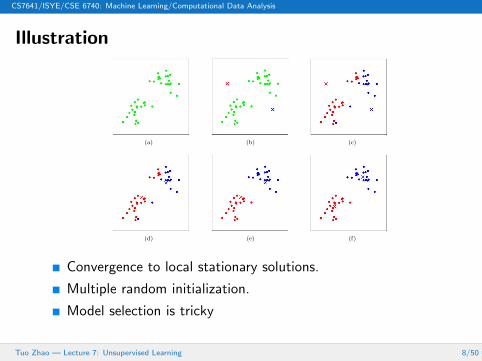
Illustration 2
(a) (b) (c)
(d) (e) (f)
Figure 1: K-means algorithm. Training examples are shown as dots, andcluster centroids are shown as crosses. (a) Original dataset. (b) Random ini-tial cluster centroids (in this instance, not chosen to be equal to two trainingexamples). (c-f) Illustration of running two iterations of k-means. In eachiteration, we assign each training example to the closest cluster centroid(shown by “painting” the training examples the same color as the clustercentroid to which is assigned); then we move each cluster centroid to themean of the points assigned to it. (Best viewed in color.) Images courtesyMichael Jordan.
Is the k-means algorithm guaranteed to converge? Yes it is, in a certainsense. In particular, let us define the distortion function to be:
J(c, µ) =m!
i=1
||x(i) − µc(i)||2
Thus, J measures the sum of squared distances between each training exam-ple x(i) and the cluster centroid µc(i) to which it has been assigned. It canbe shown that k-means is exactly coordinate descent on J . Specifically, theinner-loop of k-means repeatedly minimizes J with respect to c while holdingµ fixed, and then minimizes J with respect to µ while holding c fixed. Thus,J must monotonically decrease, and the value of J must converge. (Usu-ally, this implies that c and µ will converge too. In theory, it is possible for
Convergence to local stationary solutions.
Multiple random initialization.
Model selection is tricky
Tuo Zhao — Lecture 7: Unsupervised Learning 8/50

CS7641/ISYE/CSE 6740: Machine Learning/Computational Data Analysis
Hierarchical K-means
Hierarchical Training
Efficient Information Retrieval
Tuo Zhao — Lecture 7: Unsupervised Learning 9/50

Model-based Clustering

CS7641/ISYE/CSE 6740: Machine Learning/Computational Data Analysis
Mixture Models
Generative View:
Y ∼ Bernoulli(π)
P(Y = y) = πy(1− π)1−y
P(X = x|Y = 0) = p(x;θ0)
P(X = x|Y = 1) = p(x;θ1)
P(X = x) = π · p(x;θ1) + (1− π)p(x;θ0)
Examples: Mixture of Gaussian Distributions
The same models as Generative Learning.
Tuo Zhao — Lecture 7: Unsupervised Learning 11/50

CS7641/ISYE/CSE 6740: Machine Learning/Computational Data Analysis
Mixture of Two Gaussian Distributions
Tuo Zhao — Lecture 7: Unsupervised Learning 12/50

CS7641/ISYE/CSE 6740: Machine Learning/Computational Data Analysis
Mixture Models (K > 2)
Generative View:
Y ∼ Multinomial(π,K)
P(Y = k;π) = πk, whereK∑
k=1
πk = 1.
P(X = x|Y = k;θk) = pk(x;θk)
P(X = x; Θ) =∑K
k=1 πkpk(x;θk)
Note that fk’s can be different parametric distributions.
MLE: (π, Θ) = arg maxπk,θk
n∑
i=1
log
K∑
k=1
πkpk(xi;θk)
Tuo Zhao — Lecture 7: Unsupervised Learning 13/50

Expectation Maximization Algorithm

CS7641/ISYE/CSE 6740: Machine Learning/Computational Data Analysis
EM Algorithm as Heuristics
Suppose that we know the labels yi’s.
Parameter estimation by MLE
(π, Θ) = arg maxπk,θk
n∑
i=1
log p(xi;θyi) + log p(yi;π)
We have
πk =
n∑
i=1
1(yi = k);
θk = arg maxθk
n∑
i=1
1(yi = k) log p(xi;θk)
If not know yi’s, just estimate them.
Tuo Zhao — Lecture 7: Unsupervised Learning 15/50

CS7641/ISYE/CSE 6740: Machine Learning/Computational Data Analysis
EM Algorithm as Heuristics
At the (t+ 1)-th iteration, we take
E-Step: Compute P(y(t+1)i |xi) using the current model:
P(y(t+1)i = k|xi;π(t),Θ(t)) =
p(xi|yi = k;θ(t)k )π
(t)k∑K
k=1 p(xi|yi = j;θ(t)j )π
(t)j
.
M-Step: Compute θ(t+1)k by maximizing the expected
likelihood (taking expectation over yi’s):
Θ(t+1) = arg maxθk
n∑
i=1
K∑
j=1
P(y(t+1)i = k|xi;π(t),Θ(t)) log p(xi;θk),
π(t+1)k =
n∑
i=1
P(y(t+1)i = k|xi;π(t),Θ(t)).
Tuo Zhao — Lecture 7: Unsupervised Learning 16/50

CS7641/ISYE/CSE 6740: Machine Learning/Computational Data Analysis
Jessen’s Inequality
Given a convex function f , we have p(EX) ≤ Ep(X).
Tuo Zhao — Lecture 7: Unsupervised Learning 17/50

CS7641/ISYE/CSE 6740: Machine Learning/Computational Data Analysis
Likelihood with Latent Variables
The likelihood is given
L(Θ) =
n∑
i=1
log p(xi; Θ)
=
n∑
i=1
log
K∑
y=1
p(xi, y;θy)
=
n∑
i=1
log
K∑
y=1
qi(y)p(xi, y;θy)
qi(y)
≥n∑
i=1
K∑
y=1
qi(y) logp(xi, y;θy)
qi(y),
where∑K
y=1 qi(y) = 1.
Tuo Zhao — Lecture 7: Unsupervised Learning 18/50
CS7641/ISYE/CSE 6740: Machine Learning/Computational Data Analysis
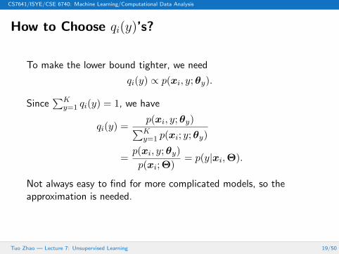
How to Choose qi(y)’s?
To make the lower bound tighter, we need
qi(y) ∝ p(xi, y;θy).
Since∑K
y=1 qi(y) = 1, we have
qi(y) =p(xi, y;θy)∑Ky=1 p(xi; y;θy)
=p(xi, y;θy)
p(xi; Θ)= p(y|xi,Θ).
Not always easy to find for more complicated models, so theapproximation is needed.
Tuo Zhao — Lecture 7: Unsupervised Learning 19/50

CS7641/ISYE/CSE 6740: Machine Learning/Computational Data Analysis
Stochastic Gradient EM Algorithm
At the (t+ 1)-th iteration, we sample i from 1, ..., n with equalprobability, or mini-batch:
E-Step: Compute P(y(t+1)i |xi) for the i-th sample only.
M-Step: Compute θ(t+1)k by stochastic gradient update:
Θ(t+1) = Θ(t) + η∇Θ`i(Θ(t)),
π(t+1)k = Πsimplex(π
(t+1)k + η∇πgi(π(t)));
where `i(Θ) and gi(π) are defined as
`i(Θ) =∑K
j=1 P(y(t+1)i = k|xi;π(t),Θ(t)) log p(xi;θk)
gi(π) =∑K
j=1 P(y(t+1)i = k|xi;π(t),Θ(t)) log πj
Tuo Zhao — Lecture 7: Unsupervised Learning 20/50

Principal Component Analysis

CS7641/ISYE/CSE 6740: Machine Learning/Computational Data Analysis
Dimensionality Reduction
Find Y = T (X), where X ∈ Rd, Y ∈ Rr and r < d.
Tuo Zhao — Lecture 7: Unsupervised Learning 22/50

CS7641/ISYE/CSE 6740: Machine Learning/Computational Data Analysis
Linear Dimensionality Reduction
Find Y = U>X, where X ∈ Rd, Y ∈ Rr and U ∈ Rd×r.
Tuo Zhao — Lecture 7: Unsupervised Learning 23/50

CS7641/ISYE/CSE 6740: Machine Learning/Computational Data Analysis
Projection to RGiven x1, ...,xn, we want to find u ∈ Rd such that
u = arg maxu
n∑
i=1
(u>xi − u>µ)2.
Why maximize the variation after projection?
Is it a well-defined problem?
`2 sphere or ball?
u = arg maxu
n∑
i=1
(u>xi − u>µ)2,
subject to ‖u‖2 = 1??
subject to ‖u‖2 ≤ 1??
Tuo Zhao — Lecture 7: Unsupervised Learning 24/50

CS7641/ISYE/CSE 6740: Machine Learning/Computational Data Analysis
Projection to Rr
Given x1, ...,xn, we want to find u1, ..., ur,∈ Rd such that
(u1, ..., ur) = arg maxu1,...,ur
r∑
j=1
n∑
i=1
(u>j xi − u>j µ)2
subject to ‖u1‖2 = 1, ..., ‖ur‖2 = 1.
Is it a well-defined problem? u1 = ... = ur.
Orthogonal constraints:
(u1, ..., ur) = arg maxu1,...,ur
r∑
j=1
n∑
i=1
(u>j xi − u>j µ)2
subject to ‖u1‖2 = 1, ..., ‖ur‖2 = 1,
u>j uk = 0 for all j 6= k.
Tuo Zhao — Lecture 7: Unsupervised Learning 25/50

CS7641/ISYE/CSE 6740: Machine Learning/Computational Data Analysis
Projection to Rr
Given X ∈ Rn×d, we want to find U ∈ Rd×r such that
U = arg maxU
Trace(U>X>
XU)
subject to U>U = I,
where X = X− 1n11>X.
X is also called centered data matrix.
Variation → Covariance?
Distributional Assumption.
Tuo Zhao — Lecture 7: Unsupervised Learning 26/50

CS7641/ISYE/CSE 6740: Machine Learning/Computational Data Analysis
Population Problem
Suppose that X ∈ Rd is a random vector with mean µ∗ andcovariance matrix Σ∗.
U∗ = arg maxU
Trace(U>Σ∗U)
subject to U>U = I,
where λr(Σ) > λr+1(Σ).
Why do we need such a gap of eigenvalues?
Is U∗ unique? Up to rotation.
Distributional Assumption.
Tuo Zhao — Lecture 7: Unsupervised Learning 27/50
CS7641/ISYE/CSE 6740: Machine Learning/Computational Data Analysis
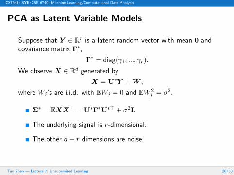
PCA as Latent Variable Models
Suppose that Y ∈ Rr is a latent random vector with mean 0 andcovariance matrix Γ∗,
Γ∗ = diag(γ1, ..., γr).
We observe X ∈ Rd generated by
X = U∗Y +W ,
where Wj ’s are i.i.d. with EWj = 0 and EW 2j = σ2.
Σ∗ = EXX> = U∗Γ∗U∗> + σ2I.
The underlying signal is r-dimensional.
The other d− r dimensions are noise.
Tuo Zhao — Lecture 7: Unsupervised Learning 28/50

CS7641/ISYE/CSE 6740: Machine Learning/Computational Data Analysis
Which r to choose?
The Signal Noise Ratio is large, Trace(Γ∗) + rσ2 (d− r)σ2.
Tuo Zhao — Lecture 7: Unsupervised Learning 29/50

CS7641/ISYE/CSE 6740: Machine Learning/Computational Data Analysis
Which r to choose?
When the SNR is not sufficiently large, it may be difficult to tell.
Tuo Zhao — Lecture 7: Unsupervised Learning 30/50

CS7641/ISYE/CSE 6740: Machine Learning/Computational Data Analysis
SVD on X
The centered data matrix X ∈ Rn×d has a SVD:
X = UDV>.
where n > d, U>U = I, V>V = I, D = diag(δ1, ..., δd), and
δ1 ≥ ... ≥ δd.
= X U V> D
Tuo Zhao — Lecture 7: Unsupervised Learning 31/50

CS7641/ISYE/CSE 6740: Machine Learning/Computational Data Analysis
SVD on X
= X V>UD
The first r columns of V are the loading vectors.
The first r columns of UD are the principal components.
Intuition of matrix factorization in machine learning.
Tuo Zhao — Lecture 7: Unsupervised Learning 32/50

CS7641/ISYE/CSE 6740: Machine Learning/Computational Data Analysis
SVD on X
= X V>UD
The first r columns of V are the loading vectors.
The first r columns of UD are the principal components.
Intuition of matrix factorization in machine learning.
Tuo Zhao — Lecture 7: Unsupervised Learning 33/50

CS7641/ISYE/CSE 6740: Machine Learning/Computational Data Analysis
PCA as Nonconvex Optimization
Recall that we solve
U = arg maxU
Trace(U>ΣU)
subject to U>U = I,
where Σ is the sample covariance matrix.
The orthogonal constraint is nonconvex.
The optimal solution can be find by SVD: O(d3).
Power Iterations:
U(t+1) = Orth(ΣU(t)) Cost : O(rd2 log ε−1
λk − λk+1
)
Tuo Zhao — Lecture 7: Unsupervised Learning 34/50

CS7641/ISYE/CSE 6740: Machine Learning/Computational Data Analysis
PCA as Nonconvex Stochastic Optimization
Recall that we solve
U = arg maxU
⟨EΣ,U>U
⟩subject to U>U = I,
where EΣ = Σ and∥∥∥Σ− Σ
∥∥∥2
2<∞.
At the (t+ 1)-th iteration, we randomly sample i and j from1, ..., n with equal probability, and have
Σ(t)
= (xi − xj)(xi − xj)> and Ei,jΣ(t)
= Σ.
Let ηt be the step size parameter. We take
U(t+1) = Orth(U(t) + ηtΣ(t)
U(t)).
Tuo Zhao — Lecture 7: Unsupervised Learning 35/50

CS7641/ISYE/CSE 6740: Machine Learning/Computational Data Analysis
PCA as Convex Stochastic Optimization
We reparametrize M = UU>, and solve
M = arg maxM
⟨EΣ,M
⟩
subject to Trace(M) = r, I M 0.
At the (t+ 1)-th iteration, we take
M(t+1) = ΠFantope
(M(t) + ηtΣ
(t)),
where ΠFantope(·) is the Fantope projection operator defined as
ΠFantope(A) = arg minB
‖A−B‖2Fsubject to Trace(B) = r, I B 0.
Tuo Zhao — Lecture 7: Unsupervised Learning 36/50

CS7641/ISYE/CSE 6740: Machine Learning/Computational Data Analysis
Nonconvex v.s. Convex Optimization
Convex Optimization:
Computationally expensive projection;
Only output an approximate low rank solution;
Slower rate of convergence:
T = O(r log d
ε2log
(1
ε
))s.t. f(M)− f(M(T )) ≤ ε.
Nonconvex Optimization:
Efficient orthogonal transformation;
Output a low rank solution;
Faster rate of convergence:
T = O(
r log d
(λr − λr+1)εlog
(1
ε
))s.t. sin2(U,U(T )) ≤ ε.
Tuo Zhao — Lecture 7: Unsupervised Learning 37/50

CS7641/ISYE/CSE 6740: Machine Learning/Computational Data Analysis
Potential of Nonconvex Optimization
Computationally intractable, but only in the worst case;
Very flexible and important in machine learning;
Very efficient in practice when well designed;
Machine learning is interested in generalization, not globaloptimal solution;
Some nonconvex problems are solvable.
Tuo Zhao — Lecture 7: Unsupervised Learning 38/50

CS7641/ISYE/CSE 6740: Machine Learning/Computational Data Analysis
Saddle Point
Tuo Zhao — Lecture 7: Unsupervised Learning 39/50

CS7641/ISYE/CSE 6740: Machine Learning/Computational Data Analysis
Quasi-Convexity
Tuo Zhao — Lecture 7: Unsupervised Learning 40/50

CS7641/ISYE/CSE 6740: Machine Learning/Computational Data Analysis
(Approximately) Equivalent Local Optima
Tuo Zhao — Lecture 7: Unsupervised Learning 41/50

CS7641/ISYE/CSE 6740: Machine Learning/Computational Data Analysis
Sparse Principal Component Analysis
Suppose that Y ∈ Rr is a latent random vector with mean 0and diagonal covariance matrix Γ∗. We observe X ∈ Rdgenerated by
X = U∗Y +W ,
where Wj ’s are i.i.d. with EWj = 0, EW 2j = σ2, and U∗ is a
sparse matrix with many zeros.
To estimate a sparse estimator of U∗, we solve
U = arg maxU
Trace(U>ΣU)− λ |||U|||1
subject to U>U = I,
where |||U|||1 =∑
j<k |Ujk|.
Tuo Zhao — Lecture 7: Unsupervised Learning 42/50

Matrix Completion

CS7641/ISYE/CSE 6740: Machine Learning/Computational Data Analysis
NETFLIX: Low Rank Matrix Completion
Tuo Zhao — Lecture 7: Unsupervised Learning 44/50

CS7641/ISYE/CSE 6740: Machine Learning/Computational Data Analysis
Matrix Factorization of M
= Rating User
Movie
M V>U
V is the movie matrix.
U is the user matrix.
Confounding factors: movie genre, time of release, etc.
Tuo Zhao — Lecture 7: Unsupervised Learning 45/50

CS7641/ISYE/CSE 6740: Machine Learning/Computational Data Analysis
NETFLIX: Low Rank Matrix Completion
Convex – Nuclear norm minimization: ‖M‖∗ =∑k
j=1 σk(M)
M = arg minM
‖M‖∗ subject to Mij = M∗ij , (i, j) ∈ Ω
Computationally inefficient;
high memory usage.
Nonconvex – Factorization minimization:
(U, V) = arg minU∈Rn×k,V∈Rm×k
∑
(i,j)∈Ω
(M∗ij − [UV>]ij)
2
Computationally efficient;
low memory usage.
Tuo Zhao — Lecture 7: Unsupervised Learning 46/50

CS7641/ISYE/CSE 6740: Machine Learning/Computational Data Analysis
Nonconvex Optimization for Matrix Completion
FixFix UV
Alternating Least Square (ALS): For t = 1, 2, ...,
U(t) = arg minU
F(U,V(t−1))
V(t) = arg minV
F(U(t),V).
Widely used in practice;
Highly efficient implementation;
For large n and m, we can apply stochastic optimization.
Tuo Zhao — Lecture 7: Unsupervised Learning 47/50

CS7641/ISYE/CSE 6740: Machine Learning/Computational Data Analysis
Robust Principal Component Analysis
We observe a matrix X ∈ Rn×d generated by
X = L∗ + S∗ + W,
where L∗ ∈ Rn×d is a rank-r matrix, and S∗ is a sparsematrix, and Wij ’s are i.i.d. with EWij = 0, EWij = σ2.
To recover L∗ and S∗, we solve a convex optimization problem
(L, S) = arg maxL,S
‖X− L− S‖2F + λ1 ‖L‖∗ + λ2 |||S|||1or nonconvex optimization problem
(U, V, S) = arg maxU,V,S
∥∥∥X−UV> − S∥∥∥
2
F+ λ |||S|||1 .
Tuo Zhao — Lecture 7: Unsupervised Learning 48/50

CS7641/ISYE/CSE 6740: Machine Learning/Computational Data Analysis
Robust PCA: Background Extraction
2 Xiao Liang, Xiang Ren, Zhengdong Zhang, Yi Ma
Fig. 1. A sample result produced by our method. Left column: input image,where the green window denotes the input window to our system. Middle column:estimated support of corruption. Right column: repaired image.
In this paper, we focus on the class of images or textures whose structureshave very low intrinsic dimensionality or complexity. More specifically we consid-er textures that when viewed as samples or signals in a high-dimensional space,span a very low-dimensional subspace or have a very sparse representation (w.r.t.certain basis). We call such textures as “Sparse Low-Rank Textures.” A directmotivation for considering such a texture model is that many regular, symmet-ric patterns commonly seen in man-made environments (e.g. building facadesand indoor decorations) are naturally sparse and low-rank. Nevertheless, thissimple texture model actually encompasses a much richer class of textures. Aswe will see, our method works equally well when the structure to be completedis not strictly periodic or stochastically stationary. In fact, our method workseven when the regular patterns are distorted by certain deformations such as anonuniform scaling or a perspective transformation – which is typically the casefor completing real images.
Another differentiating factor for image completion methods is their assump-tions about the support of the missing pixels/regions, or equivalently, what typesof missing regions they intend to handle. Are the missing pixels distributed uni-formly or clustered as blocks in the image, how large can the missing regions beor do we want to extend the texture indefinitely? The last case is often referredto as texture synthesis, which we do not consider in this paper. Actually, almostall image completion and inpainting methods need to know the exact support ofthe missing pixels, and many are very sensitive to whether the support is givenprecisely (see Figure 3 for an example). This requirement has severely limited theapplicability of image completion methods in practical scenarios. Very often wedo not know the exact pixels in an image that need to be repaired. It is desirablethat a method should be able to automatically identify and repair some corrupt-ed or occluded regions whose statistics or structures are not consistent with therest (say tree branches or a street sign blocking a building facade). When thesupport of the corrupted regions is only partially known or entirely unknown, werefer to the task as image repairing, to distinguish from the conventional imagecompletion tasks with known support.
Contributions of This Paper. In this paper, we leverage recent breakthroughs inconvex optimization for recovering sparse and low-rank structures and developeffective and efficient methods that can automatically repair sparse low-rank tex-
Tuo Zhao — Lecture 7: Unsupervised Learning 49/50

CS7641/ISYE/CSE 6740: Machine Learning/Computational Data Analysis
Robust PCA: Face Recognition
(a) M (b) L (c) S (a) M (b) L (c) S
Figure 4: Removing shadows, specularities, and saturations from face images. (a) Croppedand aligned images of a person’s face under di↵erent illuminations from the Extended YaleB database. The size of each image is 192 168 pixels, a total of 58 di↵erent illuminationswere used for each person. (b) Low-rank approximation L recovered by convex programming.(c) Sparse error S corresponding to specularities in the eyes, shadows around the nose region,or brightness saturations on the face. Notice in the bottom left that the sparse term alsocompensates for errors in image acquisition.
faces are neither perfectly convex nor Lambertian, real face images often violate this low-rankmodel, due to cast shadows and specularities. These errors are large in magnitude, but sparse inthe spatial domain. It is reasonable to believe that if we have enough images of the same face,Principal Component Pursuit will be able to remove these errors. As with the previous example,some caveats apply: the theoretical result suggests the performance should be good, but does notguarantee it, since again the error support does not follow a Bernoulli model. Nevertheless, as wewill see, the results are visually striking.
Figure 4 shows two examples with face images taken from the Yale B face database [18]. Here,each image has resolution 192 168; there are a total of 58 illuminations per subject, which westack as the columns of our matrix M 2 R32,25658. We again solve PCP with = 1/
pn1. In
this case, the algorithm requires 642 iterations to converge, and the total computation time on thesame Core 2 Duo machine is 685 seconds.
Figure 4 plots the low rank term L and the magnitude of the sparse term S obtained as thesolution to the convex program. The sparse term S compensates for cast shadows and specularregions. In one example (bottom row of Figure 4 left), this term also compensates for errors in imageacquisition. These results may be useful for conditioning the training data for face recognition, aswell as face alignment and tracking under illumination variations.
27
Tuo Zhao — Lecture 7: Unsupervised Learning 50/50


