§Even without noise§Even if the distortion is linear blur§Inverting linear blur = deconvolution
§But we want restoration to be well-posed…
6
4
A well-posed problem
§g = D( f ) is well-posed if:§For each f, a solution exists,§The solution is unique, AND§The solution g continuously depends on the data f
§Otherwise, it is ill-posed§Usually because it has a large condition number:
K >> 1
7
Condition number, K
§K » D output / D input§For the linear system b = Ax§K = ||A|| ||A-1||§K Î [1,∞)
8
5
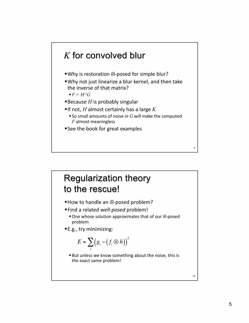
K for convolved blur
§Why is restoration ill-posed for simple blur?§Why not just linearize a blur kernel, and then take
the inverse of that matrix?§F = H-1G
§Because H is probably singular§If not, H almost certainly has a large K§ So small amounts of noise in G will make the computed
F almost meaningless§See the book for great examples
9
Regularization theoryto the rescue!§How to handle an ill-posed problem?§Find a related well-posed problem!§One whose solution approximates that of our ill-posed
problem§E.g., try minimizing:
§But unless we know something about the noise, this is the exact same problem!
10
6
Digression: Statistics
§Remember Bayes’ rule?
§p( f | g ) = p( g | f ) * p( f ) / p( g )
11
This is thea priori pdf
This is theconditional
pdf
This is thea posterioriconditional
pdf
Just anormalization
constant
This is what we want!It is our discrimination
function.
Maximum a posteriori (MAP) image processing algorithms§ To find the f underlying a given g:
1. Use Bayes’ rule to “compute all” p( fq | g )§ fq Î (the set of all possible f )
2. Pick the fq with the maximum p( fq | g )§ p( g ) is “useless” here (it’s constant across all fq)
§ This is equivalent to:§ f = argmax( fq) p( g | fq ) * p( fq )
12
Noise term Prior term
7
Probabilities of images
§Based on probabilities of pixels§For each pixel i:§p( fi | gi ) µ p( gi | fi ) * p( fi )
§Let’s simplify:§Assume no blur (just noise)§ At this point, some people would say we are denoising the image.
§p( g | f ) = ∏ p( gi | fi )§p( f ) = ∏ p( fi )
13
Probabilities of pixel values
§p( gi | fi )§This could be the density of the noise…§ Such as a Gaussian noise model§= constant * esomething
§p( fi )§This could be a Gibbs distribution…§ If you model your image as an ND Markov field
§= esomething
§See the book for more details
14
8
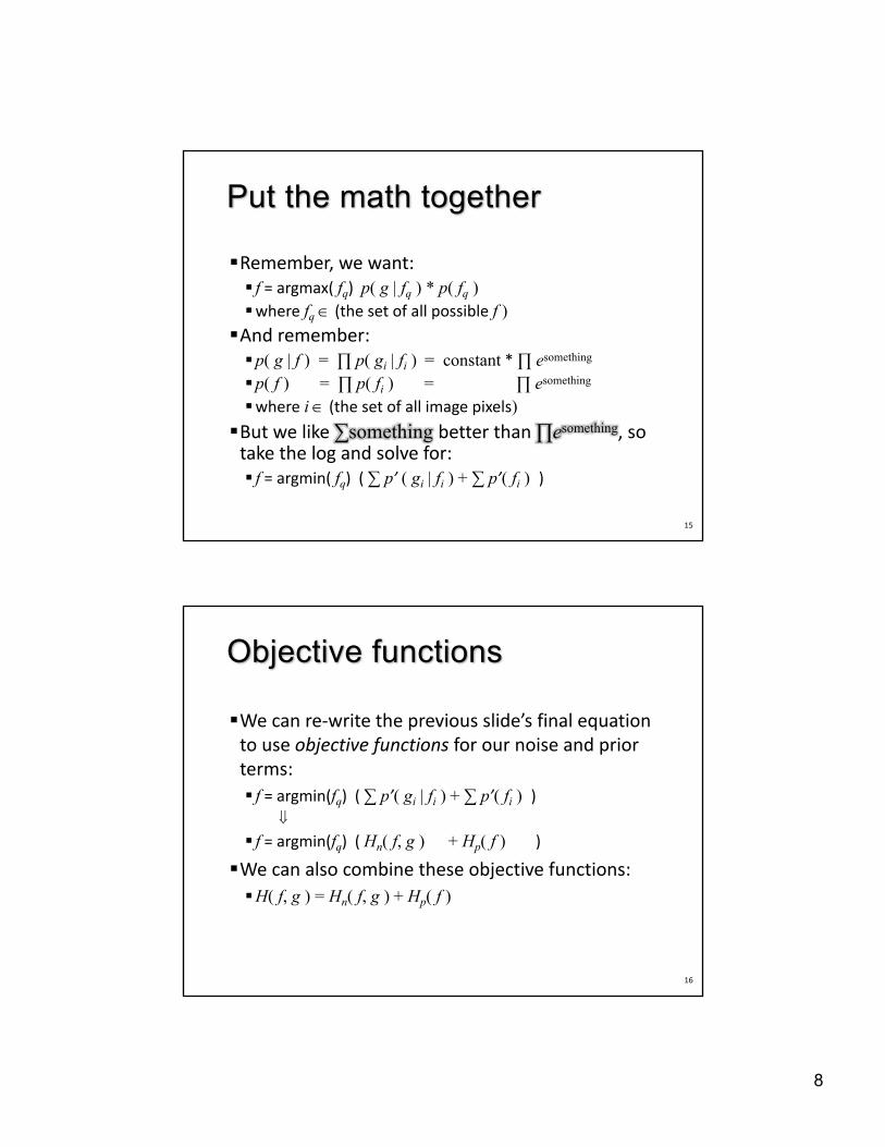
Put the math together
§Remember, we want:§ f = argmax( fq) p( g | fq ) * p( fq )§where fq Î (the set of all possible f )
§And remember:§p( g | f ) = ∏ p( gi | fi ) = constant * ∏ esomething
§p( f ) = ∏ p( fi ) = ∏ esomething
§where i Î (the set of all image pixels)§But we like ∑something better than ∏esomething, so
take the log and solve for:§ f = argmin( fq) ( ∑ p’ ( gi | fi ) + ∑ p’( fi ) )
15
Objective functions
§We can re-write the previous slide’s final equation to use objective functions for our noise and prior terms:§ f = argmin(fq) ( ∑ p’( gi | fi ) + ∑ p’( fi ) )
ß
§ f = argmin(fq) ( Hn( f, g ) + Hp( f ) )§We can also combine these objective functions:§H( f, g ) = Hn( f, g ) + Hp( f )
16
9
Purpose of the objective functions§Noise term Hn( f, g ):§ If we assume independent, Gaussian noise for each pixel,§We tell the minimization that f should resemble g.
§Prior term (a.k.a. regularization term) Hp( f ):§Tells the minimization what properties the image should
have§Often, this means brightness that is:§ Constant in local areas§ Discontinuous at boundaries
17
Minimization is a beast!
§Our objective function is not “nice”§ It has many local minima§ So gradient descent will not do well
§We need a more powerful optimizer:§Mean field annealing (MFA)§Approximates simulated annealing§But it’s faster!§ It’s also based on the mean field approximation of
statistical mechanics
18
10
MFA
§ MFA is a continuation method§ So it implements a homotopy
§ A homotopy is a continuous deformation of one hyper-surface into another
§ MFA procedure:1. Distort our complex objective function into a convex
hyper-surface (N-surface)§ The only minima is now the global minimum
2. Gradually distort the convex N-surface back into our objective function
19
0.3
0.2
0.1
0 20 40 60 80 100
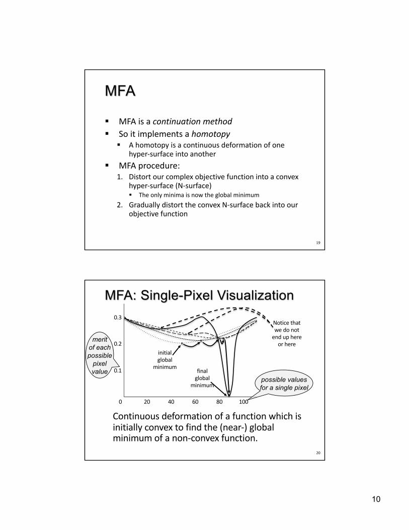
MFA: Single-Pixel Visualization
Continuous deformation of a function which is initially convex to find the (near-) global minimum of a non-convex function.
20
possible valuesfor a single pixel
meritof eachpossible
pixelvalue
initialglobal
minimum finalglobal
minimum
Notice thatwe do not
end up hereor here
11
Generalized objective functions for MFA§Noise term:
§ (D( f ))i denotes some distortion (e.g., blur) of image f in the vicinity of pixel I
§Prior term:
§ t represents a priori knowledge about the roughness of the image, which is altered in the course of MFA
§ (R( f ))i denotes some function of image f at pixel i§ The prior will seek the f which causes R( f ) to be zero (or as close to
zero as possible)
21
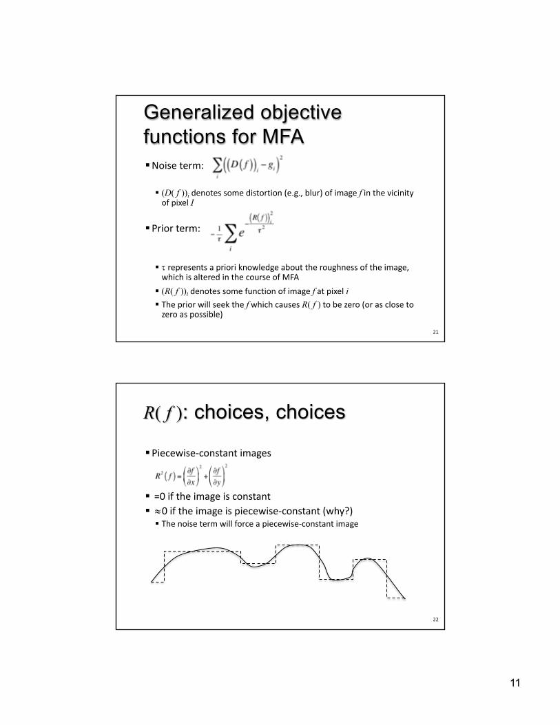
R( f ): choices, choices
§Piecewise-constant images
§ =0 if the image is constant§ »0 if the image is piecewise-constant (why?)
§ The noise term will force a piecewise-constant image
22
12
R( f ): Piecewise-planer images
§ =0 if the image is a plane§ »0 if the image is piecewise-planar
§ The noise term will force a piecewise-planar image
23
Graduated nonconvexity (GNC)
§Similar to MFA§Uses a descent method§Reduces a control parameter§Can be derived using MFA as its basis§ “Weak membrane” GNC is analogous to piecewise-
constant MFA
§But different:§ Its objective function treats the presence of edges
explicitly§ Pixels labeled as edges don’t count in our noise term§ So we must explicitly minimize the # of edge pixels
24
13
Variable conductance diffusion (VCD)
§Idea:§Blur an image everywhere,§except at features of interest§ such as edges
25
§Where:§ t = time§Ñi f = spatial gradient of f at pixel i§ ci = conductivity (to blurring)
26
VCD simulates the diffusion eq.
temporalderivative
spatialderivative
14
Isotropic diffusion
§If ci is constant across all pixels:§Isotropic diffusion§Not really VCD
§Isotropic diffusion is equivalent to convolution with a Gaussian
§The Gaussian’s variance is defined in terms of tand ci
27
VCD
§ci is a function of spatial coordinates, parameterized by i§Typically a property of the local image intensities§Can be thought of as a factor by which space is locally
compressed§To smooth except at edges:§ Let ci be small if i is an edge pixel§ Little smoothing occurs because “space is stretched” or “little heat
flows”§ Let ci be large at all other pixels§ More smoothing occurs in the vicinity of pixel i because “space is
compressed” or “heat flows easily”
28
15
VCD
§A.K.A. Anisotropic diffusion§With repetition, produces a nearly piecewise
uniform result§ Like MFA and GNC formulations§Equivalent to MFA w/o a noise term
§Edge-oriented VCD:§VCD + diffuse tangential to edges when near edges
§Biased Anisotropic diffusion (BAD)§Equivalent to MAP image restoration
29
§ From the Scientific Applications and Visualization Group at NIST§ http://math.nist.gov/mcsd/savg/software/filters/
30
VCD Sample Images
16
§Mirebeau J., Fehrenbach J., Risser L., Tobji S., “Anisotropic Diffusion in ITK”, the Insight Journal
§ Images copied per Creative Commons license§http://www.insight-journal.org/browse/publication/953
§ Then click on the “Download Paper” link in the top-right
31
Various VCD Approaches:Tradeoffs and example images
Edge Preserving Smoothing
§Other techniques constantly being developed (but none is perfect)§E.g., “A Brief Survey of Recent Edge-Preserving
Smoothing Algorithms on Digital ImagesӤhttps://arxiv.org/abs/1503.07297
§SimpleITK filters:§BilateralImageFilter§Various types of AnisotropicDiffusionImageFilter§Various types of CurvatureFlowImageFilter