Lecture 8 Mathematics of Data: ISOMAP and LLE

Lecture 8 Mathematics of Data:

ISOMAP and LLE

姚远 �

2011.4.12

John Dewey

If knowledge comes from the impressions made upon us by natural objects, it is

impossible to procure knowledge without the use of objects which impress the

mind.

Democracy and Educa.on: an introduc.on to the philosophy of educa.on, 1916

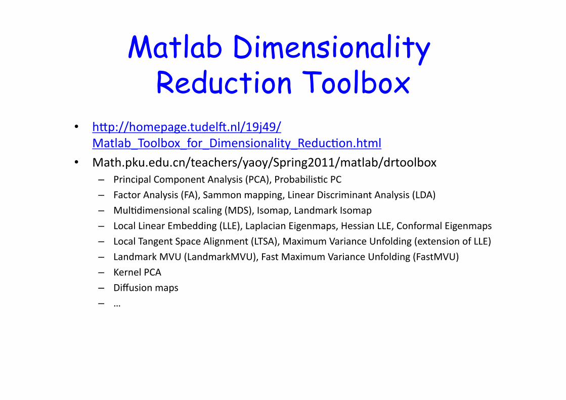
Matlab Dimensionality Reduction Toolbox

•  h#p://homepage.tudel1.nl/19j49/Matlab_Toolbox_for_Dimensionality_ReducDon.html

•  Math.pku.edu.cn/teachers/yaoy/Spring2011/matlab/drtoolbox –  Principal Component Analysis (PCA), ProbabilisDc PC

–  Factor Analysis (FA), Sammon mapping, Linear Discriminant Analysis (LDA)

–  MulDdimensional scaling (MDS), Isomap, Landmark Isomap

–  Local Linear Embedding (LLE), Laplacian Eigenmaps, Hessian LLE, Conformal Eigenmaps

–  Local Tangent Space Alignment (LTSA), Maximum Variance Unfolding (extension of LLE)

–  Landmark MVU (LandmarkMVU), Fast Maximum Variance Unfolding (FastMVU)

–  Kernel PCA

–  Diffusion maps

–  …

Recall: PCA

•  Principal Component Analysis (PCA)

One Dimensional Manifold

€

Xp×n = [X1 X2 ... Xn ]

Recall: MDS

•  Given pairwise distances D, where Dij = dij2, the squared distance between point i and j –  Convert the pairwise distance matrix D (c.n.d.) into the dot product matrix B (p.s.d.)

•  Bij (a) = -‐.5 H(a) D H’(a), Hölder matrix H(a) = I-‐1a’; •  a = 1k: Bij = -‐.5 (Dij -‐ Dik – Djk) •  a = 1/n:

–  EigendecomposiDon of B = YYT

If we preserve the pairwise Euclidean distances do we preserve the structure??

€

Bij = − 12 Dij −

1N Dsj

s=1

N

∑ − 1N Dit

t=1

N

∑ + 1N 2 Dst

s,t=1

N

∑⎛

⎝ ⎜

⎞

⎠ ⎟

Nonlinear Manifolds..

A

Unfold the manifold

PCA and MDS see the Euclidean distance

What is important is the geodesic distance

Intrinsic Description..

•  To preserve structure, preserve the geodesic distance and not the Euclidean distance.

Two Basic Geometric Embedding Methods •  Tenenbaum-de Silva-Langford Isomap Algorithm

–  Global approach. –  On a low dimensional embedding

•  Nearby points should be nearby. •  Faraway points should be faraway.

•  Roweis-Saul Locally Linear Embedding Algorithm –  Local approach

•  Nearby points nearby

Isomap •  Estimate the geodesic distance between faraway points. •  For neighboring points Euclidean distance is a good

approximation to the geodesic distance. •  For faraway points estimate the distance by a series of short hops

between neighboring points. –  Find shortest paths in a graph with edges connecting

neighboring data points

Once we have all pairwise geodesic distances use classical metric MDS

Isomap - Algorithm •  Determine the neighbors.

–  All points in a fixed radius. –  K nearest neighbors

•  Construct a neighborhood graph. –  Each point is connected to the other if it is a K nearest neighbor. –  Edge Length equals the Euclidean distance

•  Compute the shortest paths between two nodes –  Floyd’s Algorithm (O(N3)) –  Dijkstra’s Algorithm (O(kN2logN))

•  Construct a lower dimensional embedding. –  Classical MDS

Isomap

Example…

Residual Variance

Face Images SwisRoll

Hand Images 2

ISOMAP on Alanine-dipeptide Application I: Alanine-dipeptide

ISOMAP 3D embedding with RMSD metric on 3900 Kcenters

Theory of ISOMAP •  ISOMAP has provable convergence guarantees; •  Given that {xi} is sampled sufficiently dense, ISOMAP will approximate closely the original distance as measured in manifold M;

•  In other words, actual geodesic distance approximaDons using graph G can be arbitrarily good;

•  Let’s examine these theoreDcal guarantees in more detail …

Possible Issues

Two step approximaDons

Dense-‐sampling Theorem [Bernstein, de Silva, Langford, and

Tenenbaum 2000]

Proof Introduction Theoretical Claims Conformal ISOMAP Landmark ISOMAP Summary

ISOMAP Asymptotic Convergence Proofs

Proof of Theorem 1

dM(x , y) ≤ dS(x , y) ≤ (1+ 4δ/�)dM(x , y)

Proof:� The left hand side of the inequality follows directly from thetriangle inequality.

� Let γ be any piecewise-smooth arc connecting x to y with� = length(γ).

� If � ≤ �− 2δ then x and y are connected by an edge in Gwhich we can use as our path.

Global vs. Local Methods in NLDR

Proof

Proof

The Second ApproximaDon Introduction Theoretical Claims Conformal ISOMAP Landmark ISOMAP Summary


dS ≈ dG� We would like to now show the other approximate equality:dS ≈ dG. First let’s make some definitions:1. The minimum radius of curvature r0 = r0(M) is defined by

1r0 = maxγ,t �γ��(t)� where γ varies over all unit-speedgeodesics in M and t is in the domain D of γ.

� Intuitively, geodesics in M curl around ’less tightly’ thancircles of radius less than r0(M).

2. The minimum branch separation s0 = s0(M) is the largestpositive number for which �x − y� < s0 impliesdM(x , y) ≤ πr0 for any x , y ∈ M.

Lemma: If γ is a geodesic in M connecting points x and y, and if� = length(γ) ≤ πr0, then:

2r0sin(�/2r0) ≤ �x − y� ≤ �


Remarks Introduction Theoretical Claims Conformal ISOMAP Landmark ISOMAP Summary


Notes on Lemma� We will take this Lemma without proof as it is somewhattechnical and long.

� Using the fact that sin(t) ≥ t − t3/6 for t ≥ 0 we can writedown a weakened form of the Lemma:

(1− �2/24r20 )� ≤ �x − y� ≤ �

� We can also write down an even more weakened versionvalid for � ≤ πr0:

(2/π)� ≤ �x − y� ≤ �

� We can now show dG ≈ dS.


Theorem 2 [Bernstein, de Silva, Langford, and Tenenbaum 2000]

Introduction Theoretical Claims Conformal ISOMAP Landmark ISOMAP Summary


Theorem 2: Euclidean Hops ≈ Geodesic Hops

Theorem 2: Let λ > 0 be given. Suppose data pointsxi , xi+1 ∈ M satisfy:

�xi − xi+1� < s0�xi − xi+1� ≤ (2/π)r0

√24λ

Suppose also there is a geodesic arc of length � = dM(xi , xi+1)connecting xi to xi+1. Then:

(1− λ)� ≤ �xi − xi+1� ≤ �


Proof Introduction Theoretical Claims Conformal ISOMAP Landmark ISOMAP Summary


Proof of Theorem 2

� By the first assumption we can directly conclude � ≤ πr0.� This fact allows us to apply the Lemma using the weakest formcombined with the second assumption gives us:

� ≤ (π/2) �xi − xi+1� ≤ r0√24λ

� Solving for λ in the above gives: 1− λ ≤ (1− �2/24r20 ). Applyingthe weakened statement of the Lemma then gives us the desiredresult.

� Combining Theorem 1 and 2 shows dM ≈ dG. This leads us thento our main theorem...


Main Theorem [Bernstein, de Silva, Langford, and

Tenenbaum 2000]



Main TheoremTheorem 1: Let M be a compact submanifold of Rn and let {xi} be a finite setof data points in M. We are given a graph G on {xi} and positive realnumbers λ1, λ2 < 1 and δ, � > 0. Suppose:1. G contains all edges (xi , xj) of length �xi − xj� ≤ �.2. The data set {xi} statisfies a δ-sampling condition – for every point

m ∈ M there exists an xi such that dM(m, xi) < δ.3. M is geodesically convex – the shortest curve joining any two points on

the surface is a geodesic curve.4. � < (2/π)r0

√24λ1, where r0 is the minimum radius of curvature of M –

1r0

= maxγ,t �γ��(t)� where γ varies over all unit-speed geodesics in M.5. � < s0, where s0 is the minimum branch separation of M – the largest

positive number for which �x − y� < s0 implies dM(x , y) ≤ πr0.6. δ < λ2�/4.

Then the following is valid for all x , y ∈ M,(1− λ1)dM(x , y) ≤ dG(x , y) ≤ (1+ λ2)dM(x , y)


ProbabilisDc Result



Recap

� So, short Euclidean distance hops along G approximate well actualgeodesic distance as measured in M.

� What were the main assumptions we made? The biggest one was theδ-sampling density condition.

� A probabilistic version of the Main Theorem can be shown where eachpoint xi is drawn from a density function. Then the approximationbounds will hold with high probability. Here’s a truncated version of whatthe theorem looks like now:

Asymptotic Convergence Theorem: Given λ1, λ2, µ > 0 then for densityfunction α sufficiently large:

1− λ1 ≤dG(x , y)dM(x , y)

≤ 1+ λ2

will hold with probability at least 1− µ for any two data points x, y.


A Shortcoming of ISOMAP

•  One need to compute pairwise shortest path between all sample pairs (i,j) – Global – Non-‐sparse – Cubic complexity O(N3)

Locally Linear Embedding manifold is a topological space which is locally Euclidean.”

Fit Locally, Think Globally

We expect each data point and its neighbours to lie on or close to a locally linear patch of the manifold.

Each point can be written as a linear combination of its neighbors. The weights choosen to minimize the reconstruction Error.

Derivation on board

Fit Locally…

Important property... •  The weights that minimize the reconstrucDon errors are invariant to rotaDon, rescaling and translaDon of the data points. –  Invariance to translaDon is enforced by adding the constraint that the weights sum to one.

•  The same weights that reconstruct the datapoints in D dimensions should reconstruct it in the manifold in d dimensions. –  The weights characterize the intrinsic geometric properDes of each neighborhood.

Think Globally…

Algorithm (K-NN) •  Local fipng step (with centering):

– Consider a point xi – Choose its K(i) neighbors ηj whose origin is at xi – Compute the (sum-‐to-‐one) weights wij which minimizes

•  Contruct neighborhood inner product: •  Compute the weight vector wi=(wij), where 1 is K-‐vector of all-‐one and λ is a regularizaDon parameter

•  Then normalize wi to a sum-‐to-‐one vector.

€

Ψi w( ) = xi − wijη jj=1

K ( i)

∑2

, wijj∑ =1, xi = 0

€

C jk = η j ,ηk

€

wi = C + λI( )−11

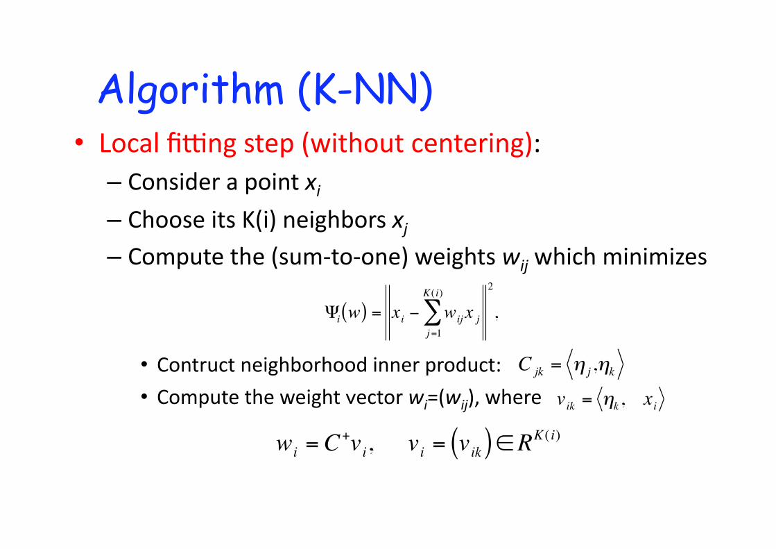
Algorithm (K-NN) •  Local fipng step (without centering):

– Consider a point xi – Choose its K(i) neighbors xj – Compute the (sum-‐to-‐one) weights wij which minimizes

•  Contruct neighborhood inner product: •  Compute the weight vector wi=(wij), where €

Ψi w( ) = xi − wij x jj=1

K ( i)

∑2

,

€

C jk = η j ,ηk

€

wi = C+vi, vi = vik( )∈RK ( i)

€

vik = ηk, xi

Algorithm continued •  Global embedding step:

– Construct N-‐by-‐N weight matrix W: – Compute d-‐by-‐N matrix Y which minimizes

•  Compute: •  Find d+1 bo#om eigenvectors of B, vn,vn-‐1,…,vn-‐d •  Let d-‐dimensional embedding Y =[ vn-‐1,vn-‐2,…vn-‐1] €

φ Y( ) = Yi − WijYjj=1

N

∑2

i∑ =Y (I −W )T (I −W )YT

€

B = (I −W )T (I −W )

€

Wij =wij , j ∈N(i)0, otherwise⎧ ⎨ ⎩

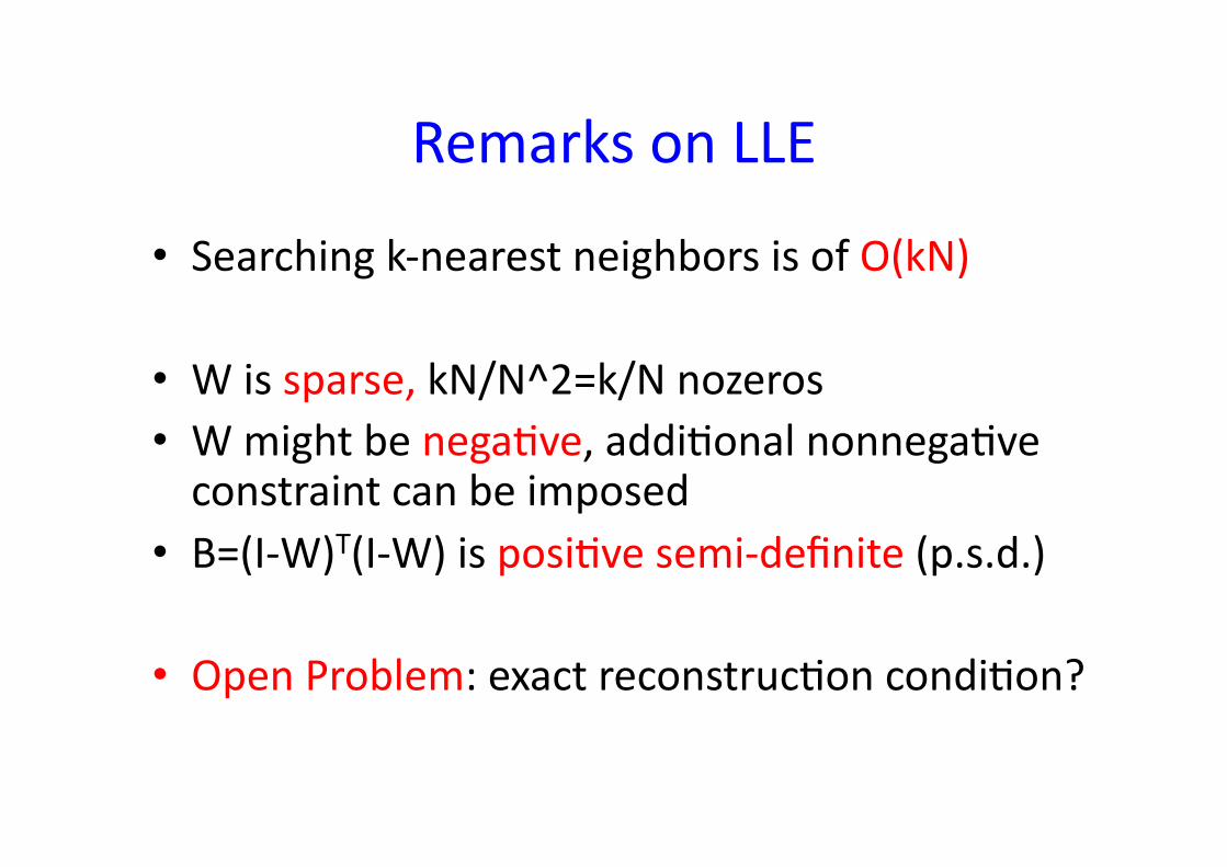
Remarks on LLE

•  Searching k-‐nearest neighbors is of O(kN)

•  W is sparse, kN/N^2=k/N nozeros •  W might be negaDve, addiDonal nonnegaDve constraint can be imposed

•  B=(I-‐W)T(I-‐W) is posiDve semi-‐definite (p.s.d.)

•  Open Problem: exact reconstrucDon condiDon?

Grolliers Encyclopedia

Summary.. ISOMAP LLE

Do MDS on the geodesic distance matrix.

Model local neighborhoods as linear a patches and then embed in a lower dimensional manifold.

Global approach Local approach

Might not work for nonconvex manifolds with holes

Nonconvex manifolds with holes

Extensions: Landmark, Conformal & Isometric ISOMAP

Extensions: Hessian LLE, Laplacian Eigenmaps etc.

Both needs manifold finely sampled.

Landmark (Sparse) ISOMAP Introduction Theoretical Claims Conformal ISOMAP Landmark ISOMAP Summary

Faster and Scalable

Motivation for L-ISOMAP� ISOMAP out of the box is not scalable. Two bottlenecks:

� All pairs shortest path - O(kN2 logN).� MDS eigenvalue calculation on a full NxN matrix - O(N3).� For contrast, LLE is limited by a sparse eigenvalue computation -O(dN2).

� Landmark ISOMAP (L-ISOMAP) Idea:� Use n << N landmark points from {xi} and compute a n x Nmatrix of geodesic distances, Dn, from each data point to thelandmark points only.

� Use new procedure Landmark-MDS (LMDS) to find a Euclideanembedding of all the data – utilizes idea of triangulation similar toGPS.

� Savings: L-ISOMAP will have shortest paths calculation ofO(knN logN) and LMDS eigenvalue problem of O(n2N).


Landmark MDS (Restriction) Introduction Theoretical Claims Conformal ISOMAP Landmark ISOMAP Summary

Faster and Scalable

LMDS Details

1. Designate a set of n landmark points.2. Apply classical MDS to the n x n matrix ∆n of the squared distances between

each landmark point to find a d-dimensional embedding of these n points. Let Lkbe the d x n matrix containing the embedded landmark points constructed byutilizing the calculated eigenvectors vi and eigenvalues λi .

Lk =

√λ1 · �vT1

√λ2 · �vT2

...

λd · �vTd


LMDS (Extension)


Faster and Scalable

LMDS Details (cont’d)

3. Apply distance-based triangulation to find a d-dimensional embedding of all Npoints.

� Let �δ1, . . . , �δn be vectors of the squared distances from the i-th landmarkto all the landmarks and let �δµ be the mean of these vectors.

� Let �δx be the vector of squared distances between a point x and thelandmark points. Then the i-th component of the embedding vector for yxis:

�y ix = −12

�vTi√λi

(�δx − �δµ)

� It can be shown that the above embedding of yx is equivalent to projectingonto the first d principal components of the landmarks.

4. Finally, we can optionally choose to run PCA to reorient our axes.


Landmark Choice Introduction Theoretical Claims Conformal ISOMAP Landmark ISOMAP Summary

Faster and Scalable

Landmark choices� How many landmark points should we choose?...� d + 1 landmarks are enough for the triangulation to locate each point uniquely,

but heuristics show that a few more is better for stability.� Poorly distributed landmarks could lead to foreshortening – projection onto the

d-dimensional subspace causes a shortening of distances.� Good methods are random OR use more expensive MinMax method that for

each new landmark added maximizes the minimum distance to the alreadychosen ones.

� Either way, running L-ISOMAP in combination with cross-validation techniqueswould be useful to find a stable embedding.


Further exploration yet… •  Hierarchical landmarks: cover-‐tree •  Nyström method

L-ISOMAP Examples


Faster and Scalable

L-ISOMAP example


Generative Models in Manifold Learning

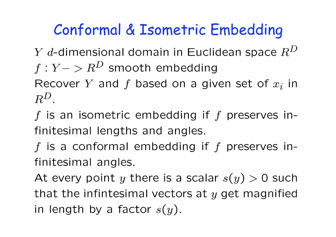
Conformal & Isometric Embedding

Isometric and Conformal •  Isometric mapping

–  Intrinsically flat manifold

–  Invariants •  Geodesic distances are reserved. •  Metric space under geodesic distance.

•  Conformal Embedding –  Locally isometric upto a scale factor s(y)

–  EsDmate s(y) and rescale. –  C-‐Isomap

–  Original data should be uniformly dense

Linear, Isometric, Conformal


Relaxing the Assumptions

Linear Isometry, Isometry, Conformal� If f is a linear isometry f : Rd → RD then we can simply use PCA or

MDS to recover the d significant dimensions – Plane.� If f is an isometric embedding f : Y → RD then provided that data

points are sufficiently dense and Y ⊆ Rd is a convex domain we canuse ISOMAP to recover the approximate original structure – Swiss Roll.

� If f is a conformal embedding f : Y → RD then we must assume thedata is uniformly dense in Y and Y ⊆ Rd is a convex domain and thenwe can successfuly use C-ISOMAP – Fish Bowl.


Conformal Isomap Introduction Theoretical Claims Conformal ISOMAP Landmark ISOMAP Summary


C-ISOMAP

� Idea behind C-ISOMAP: Not only estimate geodesicdistances, but also scalar function s(y).

� Let µ(i) be the mean distance from xi to its k-NN.� Each yi and its k-NN occupy a d-dimensional disk of radiusr – r depends only on d and sampling density.

� f maps this disk to approximately a d-dimensional disk on Mof radius s(yi)r – µ(i) ∝ s(yi).

� µ(i) is a reasonable estimate of s(yi) since it will be off by aconstant factor (uniform density assumption).


C-Isomap Introduction Theoretical Claims Conformal ISOMAP Landmark ISOMAP Summary


Altering ISOMAP to C-ISOMAP

� We replace each edge weight in G by��xi − xj

�� /�

µ(i)µ(j).Everything else is the same.

� Resulting Effect: magnify regions of high density and shrinkregions of low density.

� A similar convergence theorem as given before can be shownabout C-ISOMAP assuming that Y is sampled uniformly from abounded convex region.


C-Isomap Example I Introduction Theoretical Claims Conformal ISOMAP Landmark ISOMAP Summary


C-ISOMAP Examples Setup

� We will compare LLE, ISOMAP, C-ISOMAP, and MDS on toy datasets.� Conformal Fishbowl: Use stereographic projection to project points

uniformly distributed in a disk in R2 onto a sphere with the top removed.� Uniform Fishbowl: Points distributed uniformly on the surface of the

fishbowl.� Offset Fishbowl: Same as conformal fishbowl but points are sampled in

Y with a Gaussian offset from center.


C-Isomap Example I Introduction Theoretical Claims Conformal ISOMAP Landmark ISOMAP Summary



C-Isomap Example II Introduction Theoretical Claims Conformal ISOMAP Landmark ISOMAP Summary


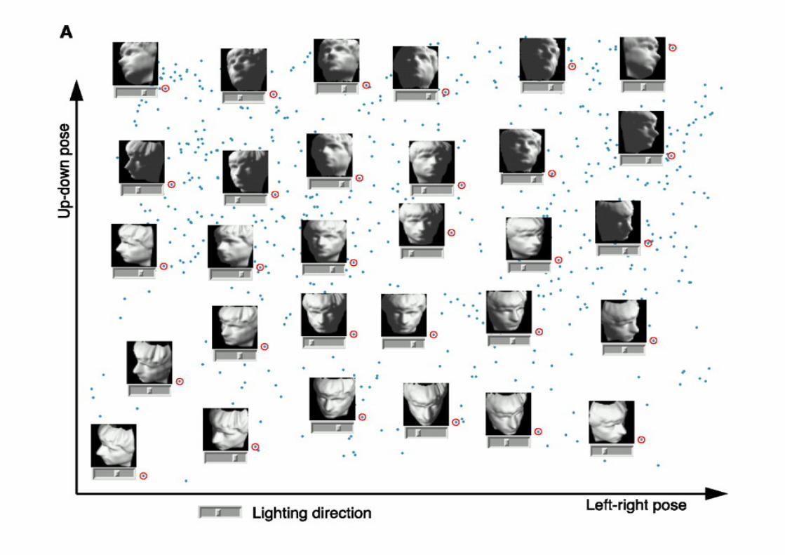
Example 2: Face Images� 2000 face images were randomly generated varying in distance and

left-right pose. Each image is a vector in 16384-dimensional space.� Below shows the four extreme cases.

� Conformal because changes in orientation at a long distance will have asmaller effect on local pixel distances than the corresponding change ata shorter distance.


C-Isomap Example II



Face Images Results

� C-ISOMAP separates the two intrinsic dimensions cleanly.� ISOMAP narrows as faces get further away.� LLE is highly distorted.


Remark

Recap and Problems Introduction Theoretical Claims Conformal ISOMAP Landmark ISOMAP Summary

Recap and QuestionsLLE ISOMAP

Approach Local GlobalIsometry Most of the time, covariance distortion YesConformal No Guarantees, but sometimes C-ISOMAPSpeed Quadratic in N Cubic in N, but L-ISOMAP

� How do LLE and L-ISOMAP compare in the quality of their output onreal world datasets? – can we develop a quantitative metric to evaluatethem?

� How much improvement in classification tasks do NLDR techniquesreally give over traditional dimensionality reduction techniques?

� Is there some sort of heuristic for choosing k? – Possibly could weutilize heirarchical clustering information in constructing a better graphG?

� Lots of research potential...


Reference

•  Tenenbaum, de Silva, and Langford, A Global Geometric Framework for Nonlinear Dimensionality ReducDon. Science 290:2319-‐2323, 22 Dec. 2000.

•  Roweis and Saul, Nonlinear Dimensionality ReducDon by Locally Linear Embedding. Science 290:2323-‐2326, 22 Dec. 2000.

•  M. Bernstein, V. de Silva, J. Langford, and J. Tenenbaum. Graph ApproximaDons to Geodesics on Embedded Manifolds. Technical Report, Department of Psychology, Stanford University, 2000.

•  V. de Silva and J.B. Tenenbaum. Global versus local methods in nonlinear dimensionality reducDon. Neural InformaDon Processing Systems 15 (NIPS’2002), pp. 705-‐712, 2003.

•  V. de Silva and J.B. Tenenbaum. Unsupervised learning of curved manifolds. Nonlinear EsDmaDon and ClassificaDon, 2002.

•  V. de Silva and J.B. Tenenbaum. Sparse mulDdimensional scaling using landmark points. Available at: h#p://math.stanford.edu/~silva/public/publicaDons.html

Acknowledgement

•  Slides stolen from Epnger, Vikas C. Raykar,Vin de Silva.

Date post:	07-Dec-2021
Category:	Documents
Upload:	others
View:	3 times
Download:	0 times

Lecture 8 Mathematics of Data: ISOMAP and LLE

Documents