41
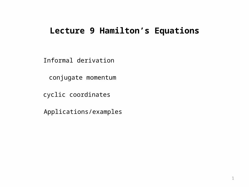
Lecture 9 Hamilton’s Equations conjugate momentum cyclic coordinates Informal derivation Applications/examples 1
| Date post: | 17-Dec-2015 |
| Category: |
Documents |
| Upload: | deborah-grant |
| View: | 238 times |
| Download: | 0 times |
1
Lecture 9 Hamilton’s Equations
conjugate momentum
cyclic coordinates
Informal derivation
Applications/examples

2
€
d
dt
∂L
∂˙ q i ⎛
⎝ ⎜
⎞
⎠ ⎟−
∂L
∂qi= λ jC1
j + Qi
Define the conjugate momentum
€
pi =∂L
∂˙ q i
Start with the Euler-Lagrange equations
€
˙ p i =∂L
∂qi+ λ jC1
j + Qi
The Euler-Lagrange equations can be rewritten as
derivation

3
If we are to set up a pair of sets of odes, we need to eliminate
€
˙ q i
We can write the Lagrangian
€
L =1
2˙ q iM ij ˙ q j −V qk
( )
M is positive definite (coming from the kinetic energy), so
€
˙ q j = M ji pi
derivation
€
pi = M ij ˙ q jfrom which

4
I have the pair of sets of odes
€
˙ q j = M ji pi
€
˙ p i =∂L
∂qi+ λ jC1
j + Qi
where all the q dots in the second set have been replaced by their expressions in terms of p
derivation

5
We can write this out in detail, although it looks pretty awful
€
L =1
2˙ q iM ij ˙ q j −V qk
( )
derivation
€
∂L
∂qi=
1
2˙ q m
∂Mmn
∂qi˙ q n −
∂V
∂qiright hand side
€
˙ q m = M mr pr, ˙ q n = M ns pssubstitute
€
∂L
∂qi=
1
2M mr pr
∂Mmn
∂qiM ns ps −
∂V
∂qiright hand side

6
€
˙ p i =∂L
∂qi+ λ jC1
j + Qi
€
∂L
∂qi=
1
2M mr pr
∂Mmn
∂qiM ns ps −
∂V
∂qi
We will never do it this way!€
˙ p i =1
2M mr pr
∂Mmn
∂qiM ns ps −
∂V
∂qi+ λ jC1
j + Qi
derivation
I will give you a recipe as soon as we know what cyclic coordinates are

7
??

8
€
˙ p i =∂L
∂qi+ λ jC1
j + Qi
If Qi and the constraints are both zero (free falling brick, say) we have
€
˙ p i =∂L
∂qi
and if L does not depend on qi, then pi is constant!
Conservation of conjugate momentum
qi is a cyclic coordinate
Given
cyclic coordinates
€
˙ p i = 0

9
YOU NEED TO REMEMBER THAT EXTERNAL FORCES
AND/OR CONSTRAINTSCAN MAKE CYCLIC COORDINATES
NON-CYCLIC!

10
??

11
What can we say about an unforced single link in general?
€
L =1
2A ˙ θ cosψ + ˙ φ sinθ sinψ( )
2+ B − ˙ θ sinψ + ˙ φ sinθ cosψ( )
2+ C ˙ ψ + ˙ φ cosθ( )
2 ⎛ ⎝ ⎜ ⎞
⎠ ⎟
+1
2m ˙ x 2 + ˙ y 2 + ˙ z 2( ) − mgz
We see that x and y are cyclic (no explicit x or y in L)
€
px = p1 = m˙ x , py = p2 = m˙ y
Conservation of linear momentum in x and y directions
We see that f is also cyclic (no explicit f in L)

12
€
pφ = p4 = Asin2ψ + Bcos2ψ( )sin2 θ + C cos2 θ( ) ˙ φ + A − B( )sinθ sinψ cosψ ˙ θ + C cosθ ˙ ψ
Does it mean anything physically?!
The conserved conjugate momentum is
the angular momentum about the k axisas I will now show you

13
The angular momentum in body coordinates is
€
l = A ˙ θ cosψ + ˙ φ sinθ sinψ( )I3 + B − ˙ θ sinψ + ˙ φ sinθ cosψ( )J3 + C ˙ ψ + ˙ φ cosθ( )IZZK 3
€
I3 = cosψ cosφI0 + sinφJ0( ) + sinψ cosθ −sinφI0 + cosφJ0( ) + sinθK 0( )
J3 = −sinψ cosφI0 + sinφJ0( ) + cosψ cosθ −sinφI0 + cosφJ0( ) + sinθK 0( )
K 3 = −sinθ −sinφI0 + cosφJ0( ) + cosθK 0
The body axes are (from Lecture 3)
and the k component of the angular momentum is
€
k ⋅l = A ˙ θ cosψ + ˙ φ sinθ sinψ( )sinψ sinθ +
B − ˙ θ sinψ + ˙ φ sinθ cosψ( )cosψ sinθ + C ˙ ψ + ˙ φ cosθ( )cosθ

14
The only force in the problem is gravity, which acts in the k direction
Any gravitational torques will be normal to k, so the angular momentum in the k direction must be conserved.
€
k ⋅l = A ˙ θ cosψ + ˙ φ sinθ sinψ( )sinψ sinθ +
B − ˙ θ sinψ + ˙ φ sinθ cosψ( )cosψ sinθ + C ˙ ψ + ˙ φ cosθ( )cosθ
€
p4 = Asin2ψ + Bcos2ψ( )sin2 θ + C cos2 θ( ) ˙ φ + A − B( )sinθ sinψ cosψ ˙ θ + C cosθ ˙ ψ
some algebra

15
Summarize our procedure so far
Write the Lagrangian
Apply holonomic constraints, if any
Assign the generalized coordinates
Find the conjugate momenta
Eliminate conserved variables (cyclic coordinates)
Set up numerical methods to integrate what is left

16
??

17
Let’s take a look at some applications of this method
Falling brick
Flipping a coin
The axisymmetric top

18
Flipping a coin

19
A coin is axisymmetric, and this leads to some simplification
€
L =1
2A ˙ θ 2 + ˙ φ 2 sin2 θ( ) + C ˙ ψ + ˙ φ cosθ( )
2
( ) +1
2m ˙ x 2 + ˙ y 2 + ˙ z 2( ) − mgz
We have four cyclic coordinates, adding y to the set and simplifying f
€
pψ = p6 = C ˙ ψ + ˙ φ cosθ( )
€
pφ = p4 = Asin2 θ + C cos2 θ( ) ˙ φ + C cosθ ˙ ψ
We can recognize the new conserved term as the angular momentum about K
€
l = A ˙ θ cosψ + ˙ φ sinθ sinψ( )I3 + B − ˙ θ sinψ + ˙ φ sinθ cosψ( )J3 + C ˙ ψ + ˙ φ cosθ( )K 3
Flipping a coin
20
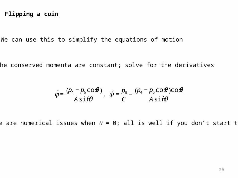
We can use this to simplify the equations of motion
€
˙ φ =p4 − p6 cosθ( )
Asin2 θ, ˙ ψ =
p6
C−
p4 − p6 cosθ( )cosθ
Asin2 θ
The conserved momenta are constant; solve for the derivatives
(There are numerical issues when q = 0; all is well if you don’t start there)
Flipping a coin

21
€
pψ = p6 = C ˙ ψ + ˙ φ cosθ( ) = 0
€
pφ = p4 = Asin2 θ + C cos2 θ( ) ˙ φ + C cosθ ˙ ψ = 0€
˙ φ = 0 = ˙ ψ
I can flip it introducing spin about I with no change in f or y
This makes p4 = 0 = p6
€
∂L
∂θ= Asinθ cosθ ˙ φ 2 − C sinθ ˙ ψ + ˙ φ cosθ( ) = 0
Then
Flipping a coin
22
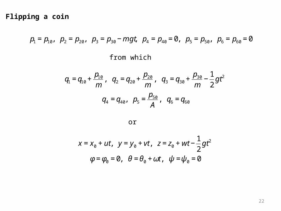
€
p1 = p10, p2 = p20, p3 = p30 − mgt, p4 = p40 = 0, p5 = p50, p6 = p60 = 0
€
q1 = q10 +p10
m, q2 = q20 +
p20
m, q3 = q30 +
p30
m−
1
2gt 2
q4 = q40, p5 =p50
A, q6 = q60
from which
€
x = x0 + ut, y = y0 + vt, z = z0 + wt −1
2gt 2
φ = φ0 = 0, θ = θ0 + ωt, ψ =ψ 0 = 0
or
Flipping a coin
23
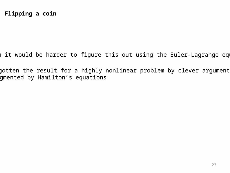
I claim it would be harder to figure this out using the Euler-Lagrange equations
Flipping a coin
I’ve gotten the result for a highly nonlinear problem by clever argumentaugmented by Hamilton’s equations

24
??

25
Same Lagrangian
but constrained
€
x
y
z
⎧
⎨ ⎪
⎩ ⎪
⎫
⎬ ⎪
⎭ ⎪= dK = d
sinφsinθ
cosφsinθ
cosθ
⎧
⎨ ⎪
⎩ ⎪
⎫
⎬ ⎪
⎭ ⎪
symmetric top
How about the symmetric top?

26
Treat the top as a cone
€
A =3
5m
1
4a2 + h2 ⎛
⎝ ⎜
⎞
⎠ ⎟= B, C =
3
10ma2
and apply the holonomic constraints
symmetric top
€
x
y
z
⎧
⎨ ⎪
⎩ ⎪
⎫
⎬ ⎪
⎭ ⎪= dK = d
sinφsinθ
cosφsinθ
cosθ
⎧
⎨ ⎪
⎩ ⎪
⎫
⎬ ⎪
⎭ ⎪

27
After some algebra
€
L =3
320m 12a2 + 31h2 + 4a2 − 31h2
( )cos 2θ( )( ) ˙ φ 2 +3
160m 4a2 + 31h2
( ) ˙ θ 2 +3
20ma2 ˙ ψ 2
3
10ma2 cosθ ˙ φ ˙ ψ −
3
4mgh cosθ
and we see that f and y are both cyclic here.
f is the rotation rate about the vertical — the precession
y is the rotation rate about K — the spin
symmetric top

28
The conjugate momenta are
€
p1 =3
160m 12a2 + 31h2
( ) + 12a2 + 31h2( )cos 2θ( )( ) ˙ φ +
3
10ma2 cosθ ˙ ψ
€
p2 =3
80m 4a2 + 31h2
( ) ˙ θ
€
p3 =3
10ma2 cosθ ˙ φ + ˙ ψ ( )
There are no external forces and no other constraints, so the first and third are conserved
symmetric top

29
We are left with two odes
€
˙ θ =80p2
3m 4a2 + 31h2( )
€
˙ p 2 = 402 p1
2 + p32
( )cosθ − p1p3 3+ cos 2θ( )( )
3m 4a2 + 31h2( )sin3 θ
+3
4mgh sinθ
The response depends on the two conserved quantitiesand these depend on the initial spin and precession rates
symmetric top
We can go look at this in Mathematica

30
Let’s go back and look at how the fall of a single brick will go in this method
Falling brick
I will do the whole thing in Mathematica

31
That’s All Folks

32
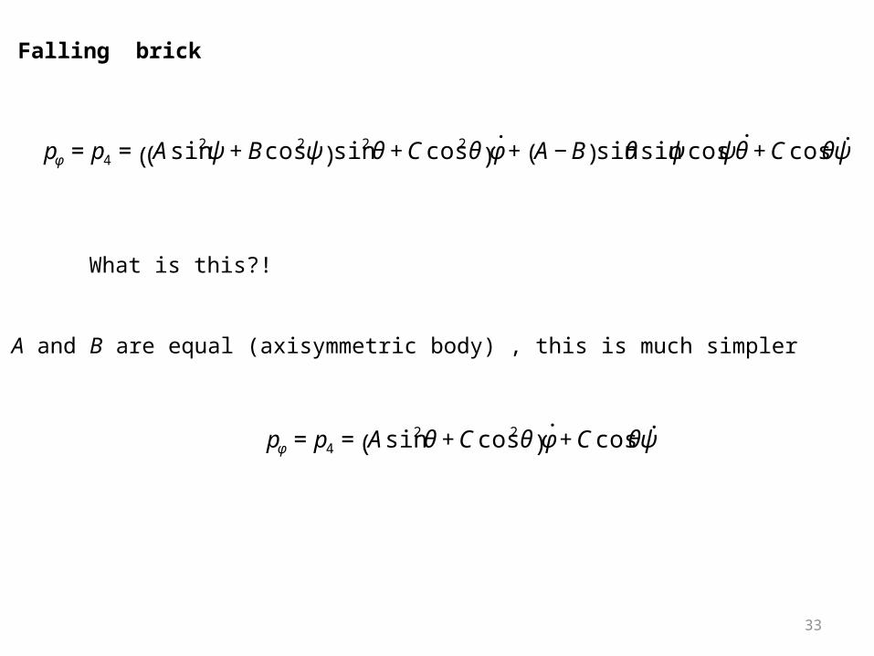
33
€
pφ = p4 = Asin2ψ + Bcos2ψ( )sin2 θ + C cos2 θ( ) ˙ φ + A − B( )sinθ sinψ cosψ ˙ θ + C cosθ ˙ ψ
What is this?!
If A and B are equal (axisymmetric body) , this is much simpler
€
pφ = p4 = Asin2 θ + C cos2 θ( ) ˙ φ + C cosθ ˙ ψ
Falling brick

34
We know what happens to all the position coordinates
All that’s left is the single equation for the evolution of p5.
After some algebra we obtain
€
˙ p 5 = −p6 − p4 cosθ( ) p4 − p6 cosθ( )
Asin3 θ
€
˙ θ =p5
A
Falling brick

35
We can restrict our attention to axisymmetric wheelsand we can choose K to be parallel to the axle
without loss of generality
€
L =1
2A ˙ θ cosψ + ˙ φ sinθ sinψ( )
2+ B − ˙ θ sinψ + ˙ φ sinθ cosψ( )
2+ C ˙ ψ + ˙ φ cosθ( )
2
( )
+1
2m ˙ x 2 + ˙ y 2 + ˙ z 2( ) − mg⋅R
€
L =1
2A ˙ θ 2 + ˙ φ 2 sin2 θ( ) + C ˙ ψ + ˙ φ cosθ( )
2
( ) +1
2m ˙ x 2 + ˙ y 2 + ˙ z 2( ) − mg⋅R
mgz
36
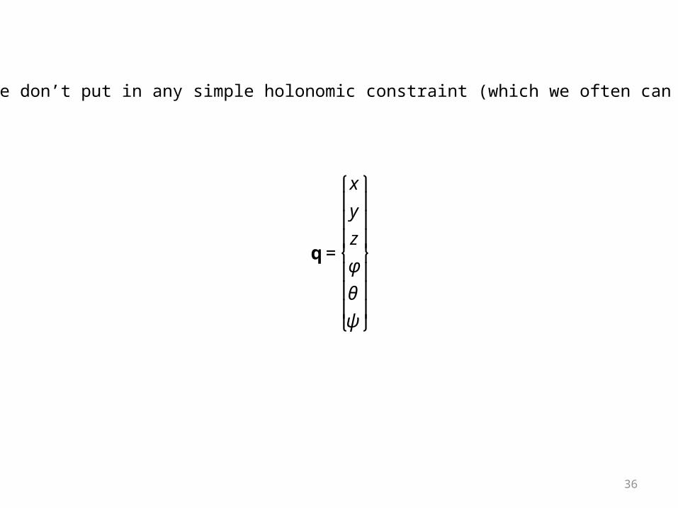
If we don’t put in any simple holonomic constraint (which we often can do)
€
q =
x
y
z
φ
θ
ψ
⎧
⎨
⎪ ⎪ ⎪
⎩
⎪ ⎪ ⎪
⎫
⎬
⎪ ⎪ ⎪
⎭
⎪ ⎪ ⎪

37
We know v and w in terms of qany difficulty will arise from r
This will depend on the surface
flat, horizontal surface — we’ve been doing this
flat surface — we can do this today
general surface: z = f(x, y) — this can be done for a rolling sphere
€
v =ω × r
€
r = −aJ2
Actually, it’s something of a question as to where the difficulties will arise in general

38
€
d
dt
∂L
∂˙ x i ⎛
⎝ ⎜
⎞
⎠ ⎟+ mgx = λ jC1
j
€
d
dt
∂L
∂ ˙ φ i ⎛
⎝ ⎜
⎞
⎠ ⎟= λ jC4
j
€
d
dt
∂L
∂ ˙ θ
⎛
⎝ ⎜
⎞
⎠ ⎟−
∂L
∂θ= λ jC5
j
€
d
dt
∂L
∂ ˙ ψ
⎛
⎝ ⎜
⎞
⎠ ⎟= λ jC6
j
€
d
dt
∂L
∂˙ y i ⎛
⎝ ⎜
⎞
⎠ ⎟+ mgy = λ jC2
j
€
d
dt
∂L
∂˙ z i ⎛
⎝ ⎜
⎞
⎠ ⎟+ mgz = λ jC3
j
39
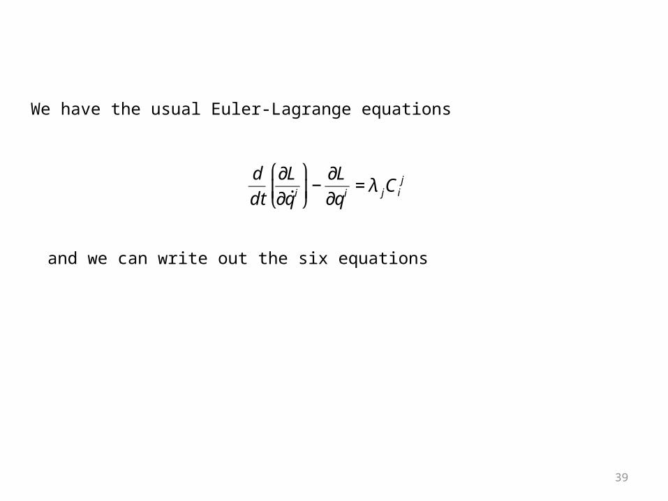
We have the usual Euler-Lagrange equations
€
d
dt
∂L
∂˙ q i ⎛
⎝ ⎜
⎞
⎠ ⎟−
∂L
∂qi = λ jCij
and we can write out the six equations
40
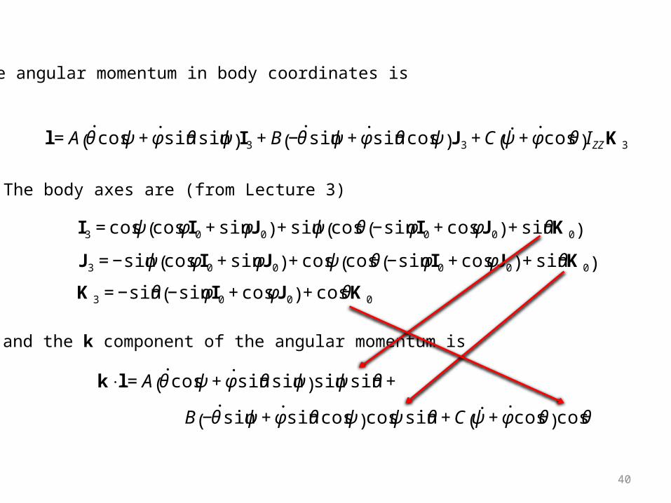
The angular momentum in body coordinates is
€
l = A ˙ θ cosψ + ˙ φ sinθ sinψ( )I3 + B − ˙ θ sinψ + ˙ φ sinθ cosψ( )J3 + C ˙ ψ + ˙ φ cosθ( )IZZK 3
€
I3 = cosψ cosφI0 + sinφJ0( ) + sinψ cosθ −sinφI0 + cosφJ0( ) + sinθK 0( )
J3 = −sinψ cosφI0 + sinφJ0( ) + cosψ cosθ −sinφI0 + cosφJ0( ) + sinθK 0( )
K 3 = −sinθ −sinφI0 + cosφJ0( ) + cosθK 0
The body axes are (from Lecture 3)
and the k component of the angular momentum is
€
k ⋅l = A ˙ θ cosψ + ˙ φ sinθ sinψ( )sinψ sinθ +
B − ˙ θ sinψ + ˙ φ sinθ cosψ( )cosψ sinθ + C ˙ ψ + ˙ φ cosθ( )cosθ

41
We will have a useful generalization fairly soonThe idea of separating the second order equations
into first order equations
€
˙ q i = M ir pr
€
˙ p i =1
2M mr pr
∂Mmn
∂qiM ns ps −
∂V
∂qi+ λ jC1
j + Qi
More generically
€
˙ q i = A ji qm( )u
j
€
˙ u i = f i qm,un( )


