Lecture 9: Introduction to Neural Networks

Refs:

Dayan & Abbott, Ch 7(Gerstner and Kistler, Chs 6, 7)D Amit & N Brunel, Cerebral Cortex 7, 232-252 (1997)C van Vreeswijk & H Sompolinsky, Science 274, 1724-1726 (1996); Neural Computation 10, 1321-1371 (1998)

Basics

N neurons, spike trains s

sjj tttS )()( ,

Basics

N neurons, spike trains s

sjj tttS )()( ,

Input current to neuron i: “current-based synapses”

j

t

jijiji tSttKtdJtI )()()(

Basics

N neurons, spike trains s

sjj tttS )()( ,

Input current to neuron i: “current-based synapses”

j

t

jijiji tSttKtdJtI )()()(

Synaptic kernel K() (normally taken indep of i,j)

Basics

N neurons, spike trains s

sjj tttS )()( ,

Input current to neuron i: “current-based synapses”

j

t

jijiji tSttKtdJtI )()()(

Synaptic kernel K() (normally taken indep of i,j)

normalization 1)(0

Kd

Basics

N neurons, spike trains s

sjj tttS )()( ,

Input current to neuron i: “current-based synapses”

j

t

jijiji tSttKtdJtI )()()(

Synaptic kernel K() (normally taken indep of i,j)

normalization 1)(0

Kd

Recall parametrization 212121

)]/exp()/[exp(1

ttPs

Basics

N neurons, spike trains s

sjj tttS )()( ,

Input current to neuron i: “current-based synapses”

j

t

jijiji tSttKtdJtI )()()(

Synaptic kernel K() (normally taken indep of i,j)

normalization 1)(0

Kd

1 presynaptic spike changes postsynaptic potential by J ij

Recall parametrization 212121

)]/exp()/[exp(1

ttPs

)( 2,1 m

Conductance-based synapses

Better:

t

jijiRj

jiji tSttKtdtVVgtI )()()]([)( 0

Differential form

For exponential kernel )/exp(1

)( ss

ttK

Differential form

For exponential kernel )/exp(1

)( ss

ttK

Differentiate => )(tSJIdt

dIj

jiji

is

Membrane potential

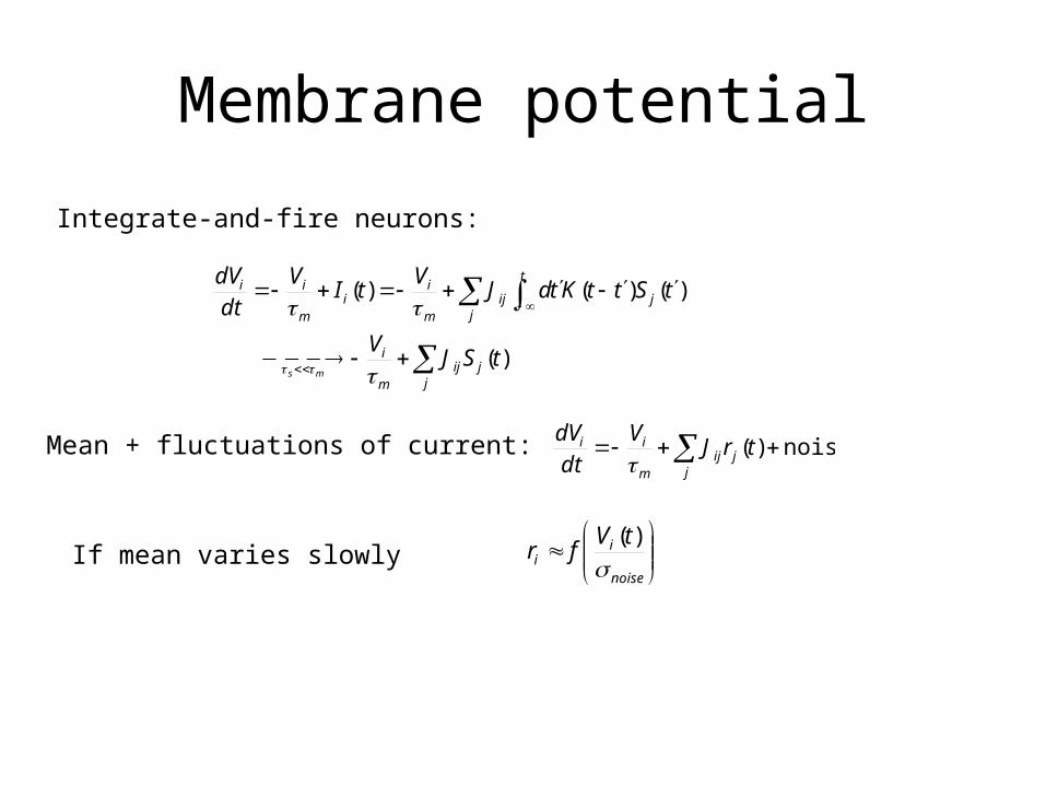
Integrate-and-fire neurons:

)(

)()()(

tSJV

tSttKtdJV

tIV

dt

dV

jj

ijm

i

t

jj

ijm

ii

m

ii

ms

Membrane potential

Integrate-and-fire neurons:

)(

)()()(

tSJV

tSttKtdJV

tIV

dt

dV

jj

ijm

i

t

jj

ijm

ii

m

ii

ms

Mean + fluctuations of current: noise)( trJV

dt

dVj

jij

m

ii

Membrane potential

Integrate-and-fire neurons:

)(

)()()(

tSJV

tSttKtdJV

tIV

dt

dV

jj

ijm

i

t

jj

ijm

ii

m

ii

ms

Mean + fluctuations of current: noise)( trJV

dt

dVj

jij

m

ii

If mean varies slowly

noise

ii

tVfr

)(

Membrane potential

Integrate-and-fire neurons:

)(

)()()(

tSJV

tSttKtdJV

tIV

dt

dV

jj

ijm

i

t

jj

ijm

ii

m

ii

ms

Mean + fluctuations of current: noise)( trJV

dt

dVj

jij

m

ii

If mean varies slowly

noise

ii

tVfr

)(

noise

j

jij

m

iiV

fJV

dt

dV

=>

Architectures

(fx retina to LGN in visual system)

Feedforward:

Architectures

(fx retina to LGN in visual system)

Feedforward:

Recurrent:

iS

j

Architectures

(fx retina to LGN in visual system)

Feedforward:

Recurrent:

iS

j

j

t

jrecijj

t

jffiji tSttKtdMtttKtdWtI )()()()()( Total input to neuron i :

Stationary statesIn limit )()( ttK

j

jijj

t

jijiji tSJtSttKtdJtI )()()()(

Stationary statesIn limit )()( ttK

j

jijj

t

jijiji tSJtSttKtdJtI )()()()(

Mean: j

jijj

jiji rJtSJtI )()(

Stationary statesIn limit )()( ttK

j

jijj

t

jijiji tSJtSttKtdJtI )()()()(

Mean: j

jijj

jiji rJtSJtI )()(

Fluctuations: )()'()()()( ttCJJtStSJJtItI jkikjk

ijkjikjk

ijii

Stationary statesIn limit )()( ttK

j

jijj

t

jijiji tSJtSttKtdJtI )()()()(

Mean: j

jijj

jiji rJtSJtI )()(

Fluctuations: )()'()()()( ttCJJtStSJJtItI jkikjk

ijkjikjk

ijii

Approximation: Assume neurons fire as independent Poisson processes:

Stationary statesIn limit )()( ttK

j

jijj

t

jijiji tSJtSttKtdJtI )()()()(

Mean: j

jijj

jiji rJtSJtI )()(

Fluctuations: )()'()()()( ttCJJtStSJJtItI jkikjk

ijkjikjk

ijii

Approximation: Assume neurons fire as independent Poisson processes:

)()( ttrttC jkjjk

Stationary statesIn limit )()( ttK

j

jijj

t

jijiji tSJtSttKtdJtI )()()()(

Mean: j

jijj

jiji rJtSJtI )()(

Fluctuations: )()'()()()( ttCJJtStSJJtItI jkikjk

ijkjikjk

ijii

Approximation: Assume neurons fire as independent Poisson processes:

)()( ttrttC jkjjk )()()( 2 ttrJtItI jj

ijii

Stationary statesIn limit )()( ttK

j

jijj

t

jijiji tSJtSttKtdJtI )()()()(

Mean: j

jijj

jiji rJtSJtI )()(

Fluctuations: )()'()()()( ttCJJtStSJJtItI jkikjk

ijkjikjk

ijii

Approximation: Assume neurons fire as independent Poisson processes:

)()( ttrttC jkjjk )()()( 2 ttrJtItI jj

ijii

Large number of inputs: Ii (t) is Gaussian

Simple model

Simple model

Input population firing at rate r0

Simple model

Input population firing at rate r0

Dilute excitatory FF connections:

cWccN

JW ijij 1probwith0,1probwith

0

0

Simple model

Input population firing at rate r0

Dilute excitatory FF connections:

cWccN

JW ijij 1probwith0,1probwith

0

0

Dilute inhibitory recurrent connections:

cMccNJ

M ijij 1probwith0,1probwith1

1

Simple model

Input population firing at rate r0

Dilute excitatory FF connections:

cWccN

JW ijij 1probwith0,1probwith

0

0

Dilute inhibitory recurrent connections:

cMccNJ

M ijij 1probwith0,1probwith1

1

1

1

0

0 ,

N

JM

N

JW

ij

ij

Simple model

Input population firing at rate r0

Dilute excitatory FF connections:

cWccN

JW ijij 1probwith0,1probwith

0

0

Dilute inhibitory recurrent connections:

cMccNJ

M ijij 1probwith0,1probwith1

1

1

1

0

0 ,

N

JM

N

JW

ij

ij

2

1

21

21

21222

20

20

20

20222

)1(

,)1(

cNJ

cNcJ

MMM

cNJ

cNcJ

WWW

ijijij

ijijij

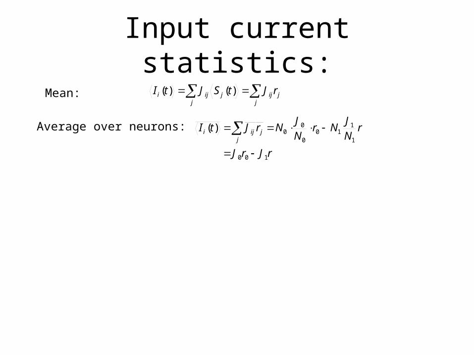
Input current statistics:

Mean: j

jijj

jiji rJtSJtI )()(

Input current statistics:

Mean: j

jijj

jiji rJtSJtI )()(

rJrJ

rNJ

NrNJ

NrJtIj

jiji

100

1

110

0

00)(

Average over neurons:

Input current statistics:

Mean: j

jijj

jiji rJtSJtI )()(

Fluctuations:

)(

)(

)()()(

1

21

0

020

21

21

1020

20

0

2

ttcN

rJcN

rJ

ttrcNJ

NrcN

JN

ttrJtItI jj

ijii

rJrJ

rNJ

NrNJ

NrJtIj

jiji

100

1

110

0

00)(

Average over neurons:

Mean field theory (white-noise approximation)

In the previous lecture, we learned how to compute the firing rate of aneuron driven by a constant current plus white noise

Mean field theory (white-noise approximation)

In the previous lecture, we learned how to compute the firing rate of aneuron driven by a constant current plus white noise

),()erf1)(exp(

,10

2/)(

/)(

0

0

IFxxdx

rI

IVrreset

Mean field theory (white-noise approximation)

In the previous lecture, we learned how to compute the firing rate of aneuron driven by a constant current plus white noise

),()erf1)(exp(

,10

2/)(

/)(

0

0

IFxxdx

rI

IVrreset

Here: use ,1000 rJrJI

Mean field theory (white-noise approximation)

In the previous lecture, we learned how to compute the firing rate of aneuron driven by a constant current plus white noise

),()erf1)(exp(

,10

2/)(

/)(

0

0

IFxxdx

rI

IVrreset

Here: use ,1000 rJrJI

1

21

0

0202

cNrJ

cN

rJ

Mean field theory (white-noise approximation)

In the previous lecture, we learned how to compute the firing rate of aneuron driven by a constant current plus white noise

),()erf1)(exp(

,10

2/)(

/)(

0

0

IFxxdx

rI

IVrreset

Here: use ,1000 rJrJI

1

21

0

0202

cNrJ

cN

rJ Solve for r

Insight from graphical solution

r

0I

Insight from graphical solution

r

0I

cNIIF

1),( 00 aroundsteep

Insight from graphical solution

r

0I rJrJI 1000

cNIIF

1),( 00 aroundsteep

Insight from graphical solution

r

r

0I rJrJI 1000

rJ1

cNIIF

1),( 00 aroundsteep

Insight from graphical solution

r

r

0I rJrJI 1000

rJ1

Root ~ at rJrJI 1000 i.e.,

cNIIF

1),( 00 aroundsteep

Insight from graphical solution

r

r

0I rJrJI 1000

rJ1

Root ~ at rJrJI 1000 i.e.,

cNIIF

1),( 00 aroundsteep

=>

0

01

0

Jr

JJ

r

Insight from graphical solution

r

r

0I rJrJI 1000

rJ1

Root ~ at rJrJI 1000 i.e.,

cNIIF

1),( 00 aroundsteep

=>

0

01

0

Jr

JJ

r Threshold-linear dependence on r0

Balance of excitation and inhibition

condition rJrJ 100

Balance of excitation and inhibition

condition rJrJ 100

Total average input current(including leak for V ~ ) = 0

Balance of excitation and inhibition

condition rJrJ 100

Total average input current(including leak for V ~ ) = 0

Balance of excitation and inhibition

condition rJrJ 100

Total average input current(including leak for V ~ ) = 0

At low rates (r << 1) membrane potentialhas to be ~ stationary below , with firingnoise-driven=> net average current = 0

Amit-Brunel model2 populations (plus external driving one)

Amit-Brunel model2 populations (plus external driving one)

indices a,b. … = 0,1,2 label populationsa = 0: externala = 1: excitatorya = 2: inhibitory

Amit-Brunel model2 populations (plus external driving one)

indices a,b. … = 0,1,2 label populationsa = 0: externala = 1: excitatorya = 2: inhibitory

Synaptic strengths:

Amit-Brunel model2 populations (plus external driving one)

indices a,b. … = 0,1,2 label populationsa = 0: externala = 1: excitatorya = 2: inhibitory

(Excitatory) external to excitatory, inhibitory ccNJ

J aaij prob,

0

00

Synaptic strengths:

Amit-Brunel model2 populations (plus external driving one)

indices a,b. … = 0,1,2 label populationsa = 0: externala = 1: excitatorya = 2: inhibitory

(Excitatory) external to excitatory, inhibitory ccNJ

J aaij prob,

0

00

Recurrent ccNJ

Jb

ababij prob,

Synaptic strengths:

Amit-Brunel model2 populations (plus external driving one)

indices a,b. … = 0,1,2 label populationsa = 0: externala = 1: excitatorya = 2: inhibitory

(Excitatory) external to excitatory, inhibitory ccNJ

J aaij prob,

0

00

Recurrent ccNJ

Jb

ababij prob,

Synaptic strengths:

2,0 bJab

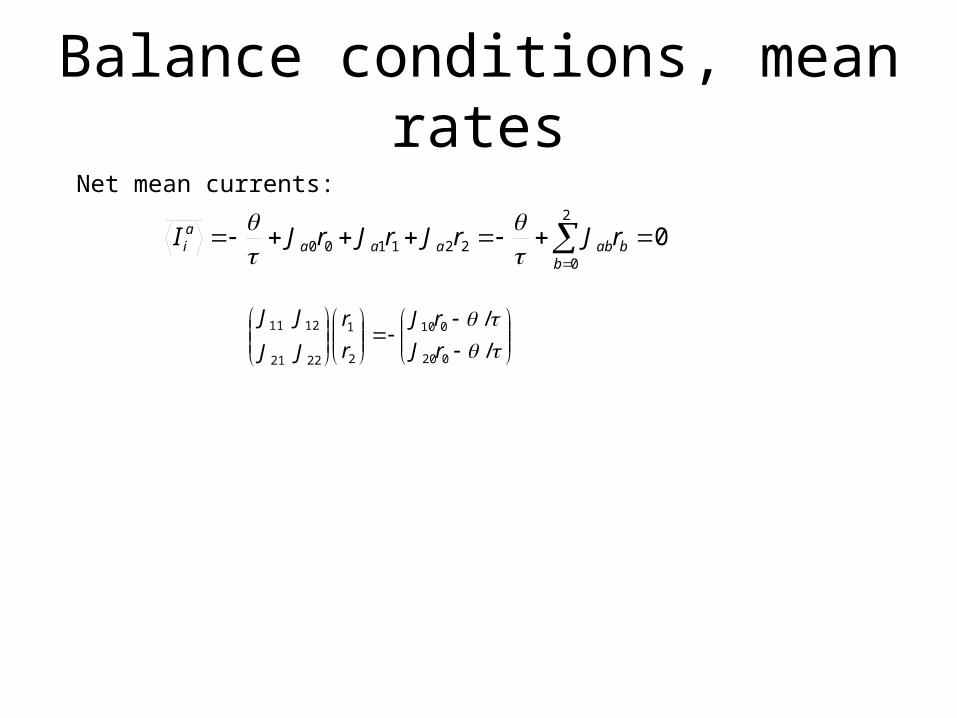
Balance conditions, mean rates

2

0221100 0

bbabaaa

ai rJrJrJrJI

Net mean currents:

Balance conditions, mean rates

2

0221100 0

bbabaaa

ai rJrJrJrJI

/

/

020

010

2

1

2221

1211

rJ

rJ

r

r

JJ

JJ

Net mean currents:

Balance conditions, mean rates

2

0221100 0

bbabaaa

ai rJrJrJrJI

Solve for r1, r2

/

/

020

010

2

1

2221

1211

rJ

rJ

r

r

JJ

JJ

Net mean currents:

Balance conditions, mean rates

2

0221100 0

bbabaaa

ai rJrJrJrJI

Solve for r1, r2

/

/

020

010

2

1

2221

1211

rJ

rJ

r

r

JJ

JJ

)(

)(

20

10

020

0101

2221

1211

2

1

J

J

rJ

rJ

JJ

JJ

r

r

Net mean currents:

Balance conditions, mean rates

2

0221100 0

bbabaaa

ai rJrJrJrJI

Solve for r1, r2

/

/

020

010

2

1

2221

1211

rJ

rJ

r

r

JJ

JJ

)(

)(

20

10

020

0101

2221

1211

2

1

J

J

rJ

rJ

JJ

JJ

r

r

Threshold-linear dependence on r0

Net mean currents: