Lecture II-1: Data Assimilation Overview

Lecture Outline:

Objectives and methods of data assimilationDefinitions and terminologyExamples

State-space formulation of the data assimilation problemState-space conceptsAccounting for uncertaintyData assimilation and estimation theory

The soil moisture data assimilation problemThe importance of soil moistureThe SGP97 field experimentProject goals and organization

What is Data Assimilation ?

Data Assimilation: Data assimilation seeks to characterize the true state of an environmental system by combining information from measurements, models, and other sources.

Typical measurements for hydrologic/earth science applications:

• Ground-based hydrologic and geological measurements (stream flow, soil moisture, soil properties, canopy properties, etc.)

• Ground-based meteorological measurements (precipitation, air temperature, humidity, wind speed, etc.)

• Remotely-sensed measurements (usually electromagnetic) which are sensitive to hydrologically relevant variables (e.g. water vapor, soil moisture, etc.)

Mathematical models used for data assimilation:

• Models of the physical system of interest.

• Models of the measurement process.

• Probabilistic descriptions of uncertain model inputs and measurement errors.

A description based on combined information should be better than one obtained from either measurements or model alone.

State estimation -- System is described in terms of state variables, which are characterized from available information

Multiple data sources -- Estimates are often derived from different types of measurements (ground-based, remote sensing, etc.) measured over a range of time and space scales

Spatially distributed dynamic systems -- Systems are often modeled with partial differential equations, usually nonlinear.

Uncertainty -- The models used in data assimilation applications are inevitably imperfect approximations to reality, model inputs may be uncertain, and measurement errors may be important. All of these sources of uncertainty need to be considered in the data assimilation process.

State variables may fluctuate over a wide range of time and space scales -- Different scales may interact (e.g. small scale variability can have large-scale consequences)

The equations used to describe the system of interest are usually discretized over time and space -- Since discretization must capture a wide range of scales the resulting number of degrees of freedom (unknowns) can be very large.

Key Features of Environmental Data Assimilation Problems

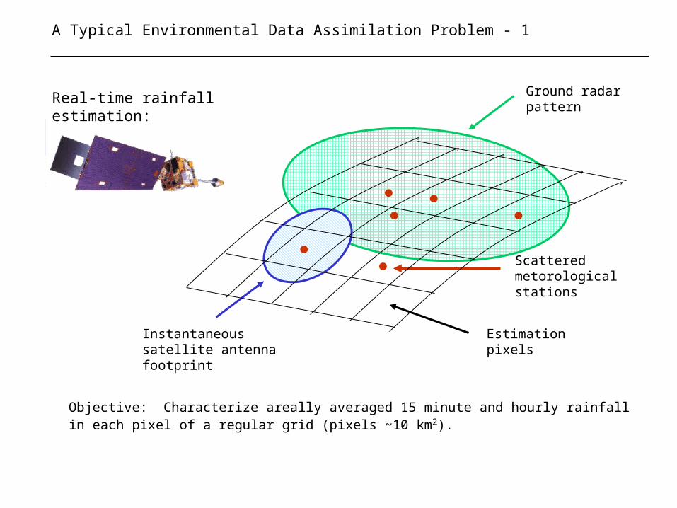
Real-time rainfall estimation:

A Typical Environmental Data Assimilation Problem - 1

Instantaneous satellite antenna footprint

Scattered metorological stations

Ground radar pattern

Estimation pixels

Objective: Characterize areally averaged 15 minute and hourly rainfall in each pixel of a regular grid (pixels ~10 km2).

Data Sources:

•Multispectral satellite data provide indirect measure of rainfall over a reasonably large area (~ 100 km2)

•Ground-based micro-meteorological data (~point data)

•Groundbased weather radar data provides another indirect measure of rainfall intensity

Models:

•Numerical weather prediction (NWP) model which relates precipitation and other state variables to atmospheric and land surface boundary conditions

•Radiative transfer models used to relate satellite and radar measurements to NWP states

•Additional measurement models which relate micro-meteorological observations to NWP states.

•Probabilitistic descriptions of inputs and measurement errors

A Typical Environmental Data Assimilation Problem - 2

In this problem we need to:

•Downscale satellite measurements (i.e. estimate rainfall at a finer spatial scale than the satellite radiobrightness measurements).

•Upscale radar measurements (i.e. estimate rainfall at a coarser spatial scale than the radar measurement pixels)

•Assimilate (or incorporate) all measurements into the NWP model (so that estimates derived from the model reflect measurements)

•Account for: Subpixel variability Model errors Measurement errors

All of this needs to be done in a systematic framework!

A Typical Environmental Data Assimilation Problem - 3

State-Space Framework for Data Assimilation

State-space concepts provide a convenient way to formulate data assimilation problems. Key idea is to describe system of interest in terms of following variables:

• Input variables -- variables which account for forcing from outside the system or system properties which do not depend on the system state.

• State variables -- dependent variables of differential equations used to describe the physical system of interest, also called prognostic variables.

• Output variables -- variables that are observed, depend on state and input variables, also called diagnostic variables.

Classification of variables depends on system boundaries:

Precip.

Land

Atmosphere

Precip.

Land

Atmosphere

System includes coupled land and atmosphere -- precipitation and evapo-transpiration are state variables

System includes only land, precipitation and evapo-transpiration are input variables

ET ET

State, Output, and Measurement Equations

State equations are intended to describe how state variables evolve over space and time. These equations are usually based on conservation laws:

)(0(0);τ],),([)( αyy 0t t ,)(u,αyAty State Eq:

Output equation relates output variables to state and input variables:

,...m ituyCtw ii 1 ; ),,,()( Output Eq:

y (), y (t) State vector (e.g. soil moisture at various locations) at times (past) and t (current)

y 0() Initial state (may depend on other inputs)

Time-invariant input vector (e.g soil conductivity at various locations)

u() Time-dependent input vector (e.g. precipitation at various locations)

w(ti) = wi Output vector at time ti (e.g. latent heat flux at various locations).

z i Measurement of w(ti)

i Measurement error at time ti

Measurement equation relates measurements to output variables:

,...m ituyMtwDz iiiiii 1 ; ],,,,[],,[ Measurement Eq:

Example: A Simple Rainfall-Runoff Model

State: Q(ti) = Streamflow

Inputs: P(ti) = Precipitation; = [1, 2 ,3 ,4]= Parameter vector

Output: S(ti) = Si = True stage

Meas: Zi = Measured stage

Error: i = Measurement error

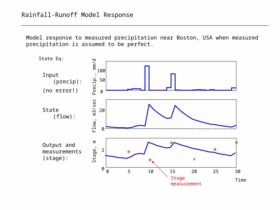
In this example, the precipitation is assumed to be perfectly known. In reality, this input will be uncertain, although a reasonable range of values may be estimated from measurements.

Consider AR(1) model of streamflow, forced by precipitation. Flow is not measured but stage is measured at selected times:

8 6, 4, 2,

9 ..., 1,

9 ..., 1,

i

i

i Q

itα

itQαaitQMiiSDiZ

αitQαaitQCiSitS

titPαitQαitPaitQAitQ

; )( 4)(3],),([],[

; 4)(3]),([)(

1 )(2)(1)](,),([)1(

; 0)( ;

State Eq:

Output Eq:

Meas. Eq:

Rainfall-Runoff Model Response

Model response to measured precipitation near Boston, USA when measured precipitation is assumed to be perfect.

0

50

100

0

20

0 5 10 15 20 25 300

2

Pre

cip.,

mm

/dFlo

w,

m3

/sec

Sta

ge,

m

Input (precip):

(no error!)

State (flow):

Output and measurements (stage): *

**

***

State Eq:

Stage measurement

Time

Deriving State-space Models for Spatially Distributed Problems - 1

Spatially distributed state-space models are typically derived by discretizing partial differential equations.

Example: 1D Saturated Groundwater Flow:

• Start with PDE derived from mass balance and Darcy’s law:

• Define piecewise linear approximations for all variables (the state y and the inputs S, T, and u). Approximations are expressed in terms of values at discrete points in time (i= 1,…,I ) and space (k = 1,…,K ):

00 ; 0),(),0( ; ),( ),(

)( ),(

)(

)y(x,txytytxu

x

txyxT

xt

txyxS K

boundary conditions

initial condition

Input (recharge)

Net inflow

Storage change

t1 tIt2

y(x, t)

At x = x1

y(x, t)

x1 xKx2

At t = t1

Deriving State-space Models for Spatially Distributed Problems - 2

• Replace derivatives by finite difference approximations at each discrete time (ti) and location (xi):

• Result is a set of K scalar state equations, one at each discrete spatial location (node). These may be assembled in a single matrix state equation:

ii

ikikik

tt

txytxy

t

txy

1

1 ),(),(

),(

kk

ikikik

xx

txytxy

x

txy

1

1 ),(),(

),(

• Similar process applies when PDE is nonlinear.

0 (0) ; )()()( 1 y tuBtyAty iii

y (ti ) = [y (x1 , ti ), y (x2 , ti ), … , y(xK , ti )]T

Accounting for Uncertainties/Errors

Uncertainties of interest in data assimilation tend to divide into:

• Structural (or “bias”) errors -- The model equations do not perfectly describe the true system (because of faulty assumptions, simplifications, approximations, omissions, etc.)

• Input uncertainties -- The model inputs are not perfectly known.

• Output uncertainties -- Output measurements differ from true outputs

)(')()( iii tPtPtP

Structural errors can sometimes be detected by examining estimates generated by the data assimilation algorithm but there is no general method for correcting such errors.

where is a known nominal (measured and or assumed) precip. and P’(ti) is the

unknown (random) difference between the true and nominal precip. values (i.e. the precip. input error).

)( itP

Input uncertainties can be accounted for if we assume that the relevant true variables are random. For example, we may assume that the true precipitation P(ti) driving the system is a random input variable given by:

Output errors are normally accounted for by including a random measurement error in the measurement equation.

100 101 1021

1.5

2

2.5

3

3.5

90 95 100 105 110 115 120-2

-1

0

1

2

3

4

Measurement error can affect observations of both model inputs and model outputs. Sources of input and output measurement error:

• Instrument errors (measurement device does not perfectly record variable it is meant to measure).

• Scale-related errors (variable measured by device is not at the same time/space scale as corresponding model variable)

Types of Measurement Errors

When measurement error statistics are specified both error sources should be considered

Large-scale trend described by model

True value

Measurement

Instrument error

Scale-related error

* *

**

Types of Data Assimilation Problems - Temporal Aspects

Zi = [z1, z2, …, zi] =Set of all measurements through time ti

Smoothing: characterize system over time interval t t i

Use for reanalysis of historic data

t t2t1 ti

Filtering/forecasting: characterize system over time interval t t i

Use for real-time forecasting

tit2t1 t

Interpolation: no time-dependence, characterize system only at time t=t i

t=ti

Use for interpolation of spatial data (e.g. kriging)

Types of Data Assimilation Problems - Spatial Aspects

Downscaling: Estimation area smaller than measurement area

Upscaling: Estimation area larger than measurement area

43211 yyyyz

Estimation areas (y1 … y4)

Measurement area (z1 )

Measurement areas (z1 ...z4)

Estimation area (y1 )

14

13

12

11

yz

yz

yz

yz

Downscaling and upscaling are handled automatically if measurement equation is defined approriately

Characterizing System States

In order to understand how each approach works we must introduce some basic concepts from probability theory. Then we can consider specific data assimilation techniques.

The basic objective of data assimilation is to characterize the true state of an environmental system (at specified times, locations, and scales). How this should be done when the states are uncertain? There are two related approaches to characterization:

• Derive a point estimate of the true state y from available information (measurements, model, error statistics)

This estimate should be “representative” of true conditions. In practice, some additional information should be provided on the range of likely values around the point estimate.

y

• Derive a range of possible values for the true state from available information. This could be conveyed in the form of a probability distribution.

This approach explicitly recognizes that we cannot perfectly identify the true state. If desired, we can select a point estimate within this range (e.g. the median).

Importance of Soil Moisture

Soil moisture is important because it controls the partitioning of water and energy fluxes at the land surface.

This effects runoff (flooding), vegetation, chemical cycles (e.g. carbon and nitrogen), and climate.

Precipitation

Runoff

Infiltration

Evapotranspiration

Soil moisture

Soil moisture varies greatly over time and space. Measurements are sparse and apply only over very small scales.

Soil moisture

Solar Radiation

Ground Heat Flux

Sensible and Latent Heat Fluxes

Microwave Measurement of Soil Moisture

L-band (1.4 GHz) microwave emissivity is sensitive to soil saturation in upper 5 cm. Brightness temperature decreases for wetter soils.

Objective is to map soil moisture in real time by combining microwave meas. and other data with model predictions (data assimilation).

0 0.2 0.4 0.6 0.8 10.5

0.6

0.7

0.8

0.9

1

saturation [-]

mic

row

ave

em

issi

vity

[-]

sandsiltclay

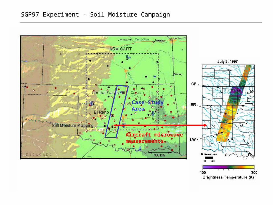
Case Study Area

Aircraft microwave measurements

SGP97 Experiment - Soil Moisture Campaign

SGP97 Experiment - Precipitation Records

Julian Day 169 =18th June 1997

170 175 180 185 190 1950

0.005

0.01

0.015

0.02

0.025

mm

/s

Precipitation at OK Mesonet Station ACME

170 175 180 185 190 1950

0.005

0.01

0.015

0.02

0.025

mm

/s

Precipitation at OK Mesonet Station ELRE

170 175 180 185 190 1950

0.005

0.01

0.015

0.02

0.025

mm

/s

Julian Day

Precipitation at OK Mesonet Station MEDF

Relevant Time and Space Scales

Vertical Section

Soil layers differ in thickness

Note large horizontal-to-vertical scale disparity

5 cm

10 cm

Typical precipitation events

For problems of continental scale we have ~ 105 est. pixels, 105 meas, 106 states,

0.8 km

0.8 km

4.0 km

Plan View

Estimation pixels (large)Microwave pixels (small)

170 = 6/19/97170 175 180 185 190 195

0

0.005

0.01

0.015

0.02

0.025

mm

/s

** ** * * * ***** ** *

* = ESTAR observation

SGP97 Experiment - Typical ESTAR Brightness Temperature Distributions

UTM

, N

4.45

4.5

4.55

4.6

4.65

65.6 5.8 6.2 6.4

80

100

120

140

160

180

200

220

240

260

3 July 9730 June 9725 June 9719 June 97 16 July 97

5.6 5.8 6 6.2 6.45.6 5.8 6 6.2 6.4 5.6 5.8 6 6.2 6.4 5.6 5.8 6 6.2 6.4 5.6 5.8 6 6.2 6.4

TB

Observing System Simulation Experiment (OSSE)

“True” radiobrightness

“Measured” radiobrightness

“True” soil moisture and temperature

Mean soil properties and land use

Land surface model (NOAH)

Mean initial conditions

Mean land-atmosphere boundary fluxes

Radiative transfer model (RTM)

Random forcing error

Random initial condition errors

Random meas. error

Data assimilation algorithm (EnKF)

Estimated microwave radiobrightness and soil moisture

Soil properties and land use, mean fluxes and initial conditions, error covariances

Estimation error

OSSE generates synthetic measurements which are then processed by the data assimilation algorithm. These measurements reflect the effect of random model and measurement errors. Performance can be measured in terms of estimation error.

Random property errors

SGP97 Project Task Summaries

The summer school project uses an OSSE to investigate a particular data assimilation algorithm (an ensemble Kalman filter) and to evaluate tradeoffs for a soil moisture satellite mission. The OSSE relies on data from the SGP97 experiment. The following three problems will be examined:

• Algorithm convergence properties -- How is convergence affected by the number of uncertain variables (error sources) included in the data assimilation algorithm?

• Identification of error statistics -- Is it possible to identify the statistical properties of model and measurement errors by observing the performance of the data assimilation algorithm?

• Mission design -- What are the best choices for satellite mission specifications such as revisit time, resolution, coverage, and accuracy? Would performance be improved by augmenting L-band microwave measurements with measurements of skin temperature?