66

Lecture Notes
Advanced Gas Dynamics
by K.V. Krasnobaev, E.I. Mogilevskiy
Contents:
conservation laws, examples of complete systems of equations; steady ow in ducts, examples of applied gas dynamics; one-dimensional wave motions, waves in compressible gas; two-dimensional steady ows, slender body linear theory; supersonic ows around blunt bodies; complicated media models.
References
Russian:
1. Êî÷èí Í.Å., Êèáåëü È. À., Ðîçå Í. Â. Òåîðåòè÷åñêàÿ ãèäðîìå-õàíèêà:  2-õ ÷./Ïîä ðåä. È. À. Êèáåëÿ. - Ì.: Ôèçìàòãèç, 1963.
2. Ëàíäàó Ë. Ä., Ëèôøèö Å. Ì. Òåîðåòè÷åñêàÿ ôèçèêà:  10-òè ò.Ò. VI. Ãèäðîäèíàìèêà. - Ì.: Íàóêà, 1986.
3. ×åðíûé Ã. Ã. Ãàçîâàÿ äèíàìèêà. - Ì.: Íàóêà, 1988.
4. Êðàñíîáàåâ Ê.Â. Ëåêöèè ïî îñíîâàì ìåõàíèêè ñïëîøíîé ñðåäû -Ì.: Ôèçìàòãèç, 2005.
English:
1. Lamb H. Hydrodynamics 6th edition, Cambridge Univ. Press. 1975
2. Liepmann H.W., Roshko A. Elements of Gas Dynamics Dover Publications,1957
3. Landau L.D., Lifshitz Theoretical physics: Vol. 6. Hydromechanics.Pergamon Press, 2nd edition, 1987.
1

Ñîäåðæàíèå
1 Basis equations 4
1.1 Mass, momentum, and energy conservation laws . . . . . . . . 41.2 Examples of complete systems of equations . . . . . . . . . . . 8
2 Lecture 2. Non-steady one- dimensional ows 10
2.1 Governing equations . . . . . . . . . . . . . . . . . . . . . . . 102.2 Small disturbances . . . . . . . . . . . . . . . . . . . . . . . . 11
3 One-dimensional nonsteady ows 15
3.1 General properties of characteristics of rst-order PDE's withtwo variables . . . . . . . . . . . . . . . . . . . . . . . . . . . 15
4 Two-dimensional steady ows 19
4.1 Governing equations. First integrals . . . . . . . . . . . . . . . 194.2 Streamfunction . . . . . . . . . . . . . . . . . . . . . . . . . . 20
5 Axisymmetric simple waves 24
5.1 General theory . . . . . . . . . . . . . . . . . . . . . . . . . . 245.2 Supersonic ow past a cone . . . . . . . . . . . . . . . . . . . 25
6 Flow past a slender body 28
6.1 Small perturbation theory . . . . . . . . . . . . . . . . . . . . 286.2 Boundary conditions . . . . . . . . . . . . . . . . . . . . . . . 30
7 Solition for potential 33
7.1 General solution . . . . . . . . . . . . . . . . . . . . . . . . . . 337.2 Examples . . . . . . . . . . . . . . . . . . . . . . . . . . . . . 357.3 Similarity rules . . . . . . . . . . . . . . . . . . . . . . . . . . 38
8 Hypersonic ows past a blunt body 43
8.1 Flow past a sphere . . . . . . . . . . . . . . . . . . . . . . . . 438.2 Basic ideas of Cherny method . . . . . . . . . . . . . . . . . . 45
9 Weak shock wave structure 48
9.1 Inviscid heat conductive gas . . . . . . . . . . . . . . . . . . . 499.2 Viscous non heat conductive gas . . . . . . . . . . . . . . . . . 51
10 Thermally non-equilibrium ows 52
10.1 Relaxation to equilibrium . . . . . . . . . . . . . . . . . . . . 5210.2 Sound propagation in a gas with relaxation . . . . . . . . . . . 53
2

10.3 Dispersion relation . . . . . . . . . . . . . . . . . . . . . . . . 5510.4 Flow in a de Laval nozzle . . . . . . . . . . . . . . . . . . . . . 57
11 Basics of nucleation theory 60
11.1 Energy barrier . . . . . . . . . . . . . . . . . . . . . . . . . . . 6011.2 Kinetics of nucleation . . . . . . . . . . . . . . . . . . . . . . . 61
3

1 Basis equations
1.1 Mass, momentum, and energy conservation laws
Consider basic equations governing motion of a medium. These equationsmathematically formulate laws based on experimental data. They are mass,momentum, and angular momentum conservation laws, rst and second lawsof thermodynamics. We postulate that these laws are valid for continuousmedia.
Derivation of the equations involves considering motion of a materialelement τ bounded by a surface Σ. For any characteristic of the mediaf(t, x, y, z) in τ , Reynolds transport theorem (the formula for time derivativeof an integral over material volume) reads
d
dt
∫τ
f dτ =
∫τ
∂f
∂tdτ +
∫Σ
fvn dΣ
(vn is the projection of the velocity vector v to the external normal vector nof the surface Σ).
If function f and velocity eld v are smooth enough, the divergencetheorem gives
d
dt
∫τ
f dτ =
∫τ
(∂f
∂t+∂fvx∂x
+∂fvy∂y
+∂fvz∂z
)dτ (1.1.1)
Consider a moving volume τ ∗ bounded by a surface Σ. Denote velocity ofthe surface points by N . For any function A(t, x, y, z) we rewrite Reynoldstransport theorem:
d
dt
∫τ∗
Adτ =
∫τ∗
∂A
∂tdτ +
∫Σ
AN dΣ .
If the volume τ ∗ coincides with a material volume τ at t = 0, we have
d
dt
∫τ
Adτ =d
dt
∫τ∗
Adτ +
∫Σ
A(vn −N) dΣ .
Continuity equation. Mass of uid in the element τ is conserved. Since(1.1.1) gives
d
dt
∫τ
ρ dτ =
∫τ
(∂ρ
∂t+∂ρvx∂x
+∂ρvy∂y
+∂ρvz∂z
)dτ = 0 (1.1.2)
4

(ρ is the gas density).As considered volume τ is arbitrary
∂ρ
∂t+∂ρvx∂x
+∂ρvy∂y
+∂ρvz∂z
= 0 (1.1.3)
The equations (1.1.2) and (1.1.3) show the mass conservation law in integraland dierential forms, respectively.
Momentum equation. By denition, momentum Q of material volumeτ is
Q =
∫τ
ρv dτ
By Newton's law, change of momentum dQ over time interval dt equalsimpulse of external forces acting on all particles inside the τ :
dQ =
∫τ
ρF dτ +
∫Σ
pndΣ
dt
where F is the mass (body) force density, and p is the stress vector. For themomentum derivative w.r.t time
dQ
dt=
∫τ
ρF dτ +
∫Σ
pndΣ
Applying (1.1.1) to the left-hand-side of this equation and taking intoaccount continuity equation, we obtain integral equation of momentum conservation.∫
τ
ρdv
dtdτ =
∫τ
ρF dτ +
∫Σ
pndΣ (1.1.4)
Cauchy formula reads
pn = px cos(n, x) + py cos(n, y) + pz cos(n, z),
and allows introducing of the stress tensor
ρdv
dt= ρF+ div Π (1.1.5)
div Π =∂px∂x
+∂py∂y
+∂pz∂z
5

Equations (1.1.4) and (1.1.5) shows the momentum conservation law inintegral and dierential forms, respectively.
For classical denition of angular momentum K
K =
∫τ
r× vρdτ
the equation (1.1.4) gives angular momentum conservation law:
dK
dt=
∫τ
r× Fρdτ +
∫Σ
r× pndΣ (1.1.6)
This law is valid for media without angular momentum corresponding tointernal degrees of freedom.
Example. Blade machines Blade machines transformmechanical energy of owing gas to kinetic energy of movingboundary (turbine) or vice versa use rotation of a rigid bodyfor gas acceleration. Gas goes through an annular duct andinteracts with blades - some plates placed across the duct.Blades are connected to a massive body in the center andthey form a rotor all together. (pic. 1).
Pic. 1: Schemeof a blademachine
Our aim is to nd power of a turbine for given ow parameters.Let ω be the angular velocity of the rotor. Consider a control volume τ ∗
bounded by the inlet Σ1, outlet Σ2 and the walls of the duct (pic. 1). Thisvolume rotates with the rotor. According (1.1.6) the angular momentumconservation law reads
d
dt
∫τ∗
(r× ρv)dτ +
∫Σ
(r× ρv)(vn −D)dΣ = ~M
~M is the principal torque, r is the position vector of some point on the ductaxis, D is the normal velocity of the surface. The parameters distributionover Σ1 are axially symmetric and the ow is steady relative to the controlvolume. So
M =
∫Σ
(r× ρv)(vn −D)dΣ
Tangential stresses on the duct walls are negligible and normal stresses givezero torque about the axis of the duct. Project this equation on the axisdirection
M =
∫Σ1+Σ2
rρcuvndΣ
6

Gas ux though boundaries is proportional to vn −D and vanishes at walls,so only integral over (Σ1 +Σ2) is non-zero. Scalar r is distance to the axis, cuis a transversal (circumferential, azimuthal) component of the absolute gasvelocity.
Power W of the rotor is
W = ωM = ω
∫Σ1+Σ2
rρcuvndΣ (1.1.7)
or
W = ω
∫ G
0
[(rcu)2 − (rcu)1]dm (1.1.8)
Here G is the total mass ux, dm is mass of the gas owing through anelement of cross-sections dΣ1 and dΣ2 of surfaces Σ1 and Σ2.
Due to mass conservation
dm = ρ1vn1dΣ1 = ρ2vn2dΣ1
and (1.1.8) has a form:
W = ω[(rcu)2 − (rcu)1]∗G (1.1.9)
The (∗) means mass average. The formula (1.1.9) was rst obtained byLeonard Euler.
The rst law of thermodynamics. There exist a variable of state E suchthat
dE = dA(e) + dQ(e)
where dA(e) is work of external forces over the system and dQ(e) is quantityof heat come from surroundings.
For a material element dτ with mass of ρdτ , E = (E + U) ρdτ , where Eis the specic kinetic energy v2/2 and U is a variable of sate, namely thespecic internal energy.
The momentum equation gives a value of a kinetic energy change, and therst law of thermodynamics leads to the equation for internal energy only(the energy equation):
dU
dt=
1
ρ
(px∂v
∂x+ py
∂v
∂y+ pz
∂v
∂z
)+ q(e) (1.1.10)
where
q(e) = limdτ→0dt→0
dQ(e)
ρdτdt
is the non-mechanical energy ux from surroundings to a unit mass of mediumper unit time.
7

The second law of thermodynamics. There exist a variable of state S(entropy) such that for reversible processes
TdS = dQ(e).
For an irreversible process leading from a state A to a state B, the secondlaw reads
S(B)− S(A) ≥∫L
dQ(e)
T.
In the right-hand-side, the integral is taken over the curve L corresponding tothe irreversible process in the conguration space. Since entropy is a variableof state S(A) and S(B) are dened independently on the path L.
1.2 Examples of complete systems of equations
One of the main problems of gas dynamics is to derive a complete systemof equations. Together with appropriate initial and boundary conditions itallows analysis of particular gas ows.
The most wide-used model is a model of ideal perfect gas. It assumesthat all mechanical processes are reversible, the stress tensor is hydrostatic(pn = −pn, p > 0), the internal energy U and pressure p depend on twovariables of state. The continuity (1.1.3), momentum (1.1.5) and energy(1.1.10) equations reads
dρ
dt+ ρdiv v = 0
ρdv
dt= ρF− grad p
dU
dt+p
ρdiv v = q(e).
(1.2.1)
Usually F and q(e) are given functions of variables involved in (1.2.1). Asthis system of equations is not complete, relations between ρ, p, U (equationsof state) must be added.
Thermic p = p(ρ, T ) (T being the temperature) and caloric U = U(ρ, T )equations of state are usually given. The functions p(ρ, T ) and U(ρ, T ) arenot independent as they must admit laws of thermodynamics.
Let the density and specic entropy be independent variables, then
U = U(ρ, s), p = p(ρ, s), T = T (ρ, s)
8

are known functions and these relations close (1.2.1). It becomes a completesystem of equations for unknowns: ρ,v, s
dρ
dt+ ρdiv v = 0
ρdv
dt= ρF− grad p
Tds
dt= q(e) .
(1.2.2)
We nd p and T by relations
p = ρ2∂U
∂ρ, T =
∂U
∂s
The model of perfect gas reads
U = cvT, p = ρRT, cv, R = const.
Hence specic entropy is
s = cv lnp
ργ+ s0, s0 = const, γ =
cv +R
cv
Introducing this expression in (1.2.2) simplies the equations and gives equationsfor ρ,v, T
dρ
dt+ ρvdiv v = 0
ρdv
dt= ρF− grad p
cvTd
dtln
(p
ργ
)= q(e)
p = ρRT.
(1.2.3)
For application, it is useful to consider gas as barotropic, i.e. p = Φ(ρ),the function Φ(ρ) is the same for any elements in considered domain.
9

2 Lecture 2. Non-steady one- dimensional ows
2.1 Governing equations
A motion is called one-dimensional if all the parameters of the media dependon one coordinate x and, in general, on time t only. If this coordinate isdistance to a certain plane the ow is plane (plane waves), if it is distanceto a straight line the ow is axisymmterical (cylindrical waves), and if itis distance to a certain point the ow is spherically symmetric (sphericalwaves). Assume, that only x component of velocity is non-zero. Body forcealso has only x non-zero component, if any.
For Eulerian description (1.2.2), unknown function are velocity componentu and two thermodynamic variables, e.g. pressure p and density ρ, while xand t are independents variables.
The continuity and motion equations reads
∂ρ
∂t+∂ρu
∂x+ (ν − 1)
ρu
x= 0 (2.1.1)
∂u
∂t+ u
∂u
∂x+
1
ρ
∂p
∂x= Fx (2.1.2)
where ν = 1, 2, 3 used for plane, cylindrical, and spherical waves, respectively.The entropy change equation is added to the systems of equations (2.1.1),
(2.1.2)
T
(∂s
∂t+ u
∂s
∂x
)= q(e) (2.1.3)
and a relation for entropy (equation of state) as well
p = p(ρ, s), T = T (ρ, s) (2.1.4)
Then, the obtained system of equation (2.1.1) (2.1.3) with additionalrelation (2.1.4) forms complete system of equations for functions u(x, t),ρ(x, t), p(x, t).
Further, we will use the continuity equation (2.1.1) in the form containingfull derivative of p over time. Since ρ = ρ(p, s), introducing speed of sound aas a2 = (∂p/∂ρ)s, from (2.1.1) we have
1
a2
(∂p
∂t+ u
∂p
∂x
)+ ρ
∂u
∂x+ (ν − 1)
ρu
x= 0 (2.1.5)
The system (2.1.1) (2.1.3) is a PDE system. So, to complete thestatement of the problem and nd a solution, initial and boundary conditionsmust be specied.
10

2.2 Small disturbances
The simplest solution for the gas dynamics equations (2.1.1) (2.1.3) describesgas in rest:
p = p0, ρ = ρ0, u = 0, s = s0, T = T (ρ0, s0)
p0, ρ0, s0 are constants.In this lecture we analyse solutions which are close to this one.Consider 1D non-stationary ows, where pressure p, density ρ slightly
dier from constant values p0, ρ0, and gas velocity u is small. The scale forvelocity comes from the gas state, it is speed of sound a0 =
√(∂p/∂ρ) s. This
velocity has the same order of magnitude as velocity of chaotic motion of gasmolecules.
Disturbances are small so p p0, ρ ρ0, u a0, s − s0 s0 andsmooth ∂/∂t a0∂/∂x. Nonlinear terms in governing equations: continuity(2.1.1), equation of motion (2.1.2) and entropy (2.1.3) can be omitted andthese equations read
∂ρ
∂t+ ρ0
∂u
∂x+ (ν − 1)
ρ0u
x= 0 (2.2.1)
∂u
∂t+
1
ρ0
∂p
∂x= 0 (2.2.2)
∂s
∂t= 0 (2.2.3)
As ρ = ρ(p, s) , we have
ρ− ρ0 =∂ρ
∂p
∣∣∣∣s
(p− p0) +∂ρ
∂s
∣∣∣∣p
s (2.2.4)
Potential ϕ integrates (2.2.2):
u =∂ϕ
∂x, p− p0 = −ρ0
∂ϕ
∂t(2.2.5)
Dierentiation of (2.2.4) w.r.t. time according (2.2.3) and (2.2.5) leads toequation for ϕ from (2.2.1):
1
a20
∂2ϕ
∂t2− ∂2ϕ
∂x2− ν − 1
x
∂ϕ
∂x= 0 (2.2.6)
11

Plane waves. For ν = 1, (2.2.6) is a classical wave equation and its generalsolution is
ϕ = F (x− a0t) +G(x+ a0t)
u = f(x− a0t) + g(x+ a0t)
p− p0 = ρ0a0 [f(x− a0t)− g(x+ a0t)]
f = F ′, g = G′
Values r = u + (p − p0)/(ρ0a0) and l = u − (p − p0)/(ρ0a0) are constanton right-running and left-running characteristics x = x0 ± a0t, respectively.This form of the solution simplies analysis of reection.
If a single pulse appears at t = 0 at some nite segment, waves go to bothdirection and their shape does not change during the propagation.
Spherical waves. For ν = 3, (2.2.6) is equivalent to
1
a20
∂2xϕ
∂t2− ∂2xϕ
∂x2= 0
It is again a wave equation, so its general solution has a form:
ϕ =1
x[F (x− a0t) +G(x+ a0t)]
Velocity and pressure are
u =f(x− a0t)
x− 1
x2
∫ x−a0t
ξ0
f(ξ)dξ +g(x+ a0t)
x− 1
x2
∫ x+a0t
η0
g(η)dη
p− p0
ρ0a0
=f(x− a0t)
x− g(x+ a0t)
x
Consider a particular solution describing pressure wave propagation awayfrom the center with potential ϕ
ϕ = − 1
4πxQ
(t− x
a0
)(2.2.7)
Velocity and pressure are
u =∂ϕ
∂x=
1
4π
Q ′(t− x
a0
)a0x
+Q(t− x
a0
)x2
p− p0 = −ρ0
∂ϕ
∂t= ρ0a0
1
4πxQ ′(t− x
a0
)12

The mass ux q(x, t) through a surface x = const is
q = 4πx2u =x
a0
Q ′(t− x
a0
)+Q
(t− x
a0
)If x→ 0
limx→0
q(x, t) = Q(t)
Let the function Q(t) in (2.2.7) is non-zeroonly if 0 < t < τ . Assume, gas comes to restafter the wave is gone. It means
Q(0) = Q ′(0) = 0, Q(τ) = Q ′(τ) = 0
As
Q(τ) =
∫ τ
0
Q ′(t)dt = 0,
the sign of Q ′(t) has to change. Consequently,the sign of pressure disturbance changes aswell. Note, that there is no such an eect forplane waves.
0
0 0.5 1 1.5 2
F1F2
0
F1F2
Q
Q'
Pic. 2: Initial disturbance
On the other hand, if pressure has a constant sign (or∫ τ
0Q ′(t)dt = Q(τ) 6=
0), gas does not come to rest but moves stationary and has velocity of
u =Q(τ)
4πx2
after the wave propagation. Anyway, both pressure and velocity have a factorof 1/x and a pulse decreases going from the center. The power of -1 ensuresenergy conservation.
Cylindrical waves. It is more dicult to derivegeneral solution for cylindrical waves then for planeof spherical ones.Consider a class of solutions which are representedas a superposition of spherical waves from uniformlydistributed over the axis x = 0 sources (pic. 3)
ϕ =
∫1
r[F (r − a0t) +G (r + a0t)] dζ,
r2 = x2 + ζ2.
(2.2.8) Pic. 3: Constructionof cylindrical wavepotential
13

Consider
F = − 1
4πQ
(t− r
a0
)and nd approriate integration limits in (2.2.8)
ϕ(t, x) = − 1
2π
∫ √a20t2−x2
0
Q(t−√x2 + ζ2/a0
)√x2 + ζ2
dζ (2.2.9)
(we took into account that z = 0 is a symmetry plane).If Q(t) is nonzero for a nite time τ , the lower limit in (2.2.9) is actually
ζterm =√a2
0(t− τ)2 − x2
if this value is greater than zero.For any xed x > 0, ϕ 6= 0 for large enough t: there always is a diapason
on the axis which contains sources giving nozero impact at a given point atany instant after rst wave come.
0
F2F1F3F4
0
0 1 2 3 4
F2F3
x
0
F2F3
p-p0
p-p0
p-p0
Pic. 4: Pressure distribution in impulse for plane, cylindrical, and sphericalwave
The pic. 4 shows pressure impulse evolution for plane, cylindrical andspherical cases. Function F (ξ) = ξ2(ξ − τ)2 is the same for all geometricalcongurations and shown at top left panel and its derivative at bottom leftone. This function denes potential. Right panels show pressure distributionin space for two instants: t = 2τ , t = 4τ , the scale for coordinate is a0τ .
Plane waves propagate without any change. Spherical waves decrease theirmagnitude while going from the origin. For symmetric in time source, the rearfront is steeper than the leading one. Single cylindrical pulse has no rear edge.At any point, pressure goes to zero during innite time.
14

3 One-dimensional nonsteady ows
3.1 General properties of characteristics of rst-order
PDE's with two variables
Consider a system of PDE's with two independent variables. Its general formis
(A)fx + (B)ft +D = 0 (3.1.1)
where (A) and (B) are matrices, D is a vector and their elements depend onx and t, and component of unknown vector-function f . The derivatives fx,ft enter the equation (3.1.1) linearly.
The system (2.1.1) (2.1.3) is an example of such a system: it is linear onderivatives of unknown functions, but its coecients and free terms dependon unknowns and independent variables arbitrary.
Consider the following problem for the equation (3.1.1). On a certain linex = x(t), values of f are given. It means that the derivative df/dt = ϕ′(t) onthis line is also given. Values fx comes from (3.1.1).
This problem is equivalent to Cauchy problem: nd a solution of (3.1.1)such that f = ϕ(t) on x = x(t). If there exists a unique solution, then fx isdetermined on x = x(t). In other words, if fx either doesn't exist or is non-unique, then the Cauchy problem either has no solution or has more thanone solution.
To obtain an equation for fx, we eliminate ft:
ϕ′(t) =∂f
∂t+dx
dt
∂f
∂xft = −dx
dtfx + ϕ′(t) (3.1.2)
Substituting ft from (3.1.2) to (3.1.1) we obtain system of linear algebraicequations for fx. If the determinant of this system is non-zero, we have aunique solution for fx on x = x(t). If
∆ =∣∣(A)− dx
dt(B)∣∣ = 0 , (3.1.3)
the system of equations for fx either has no solution or has innitelymany solutions. In the latter case, the function ϕ can not be stated arbitrary.Solvability of the system requires certain conditions for ϕ.
The equation ∆ = 0 determines directions dx/dt of characteristics.
Example 1. Find characteristics of (2.1.1) (2.1.3) with use of (2.1.4).We change (2.1.3) by the equivalent introducing speed of sound a = (∂p/∂ρ)s
∂p
∂t+ u
∂p
∂x− a2
(∂ρ∂t
+ u∂ρ
∂x
)= 0,
15

Denote
f =
ρup
, (A) =
u ρ 00 u 1/ρ−a2u 0 u
, (B) =
1 0 00 1 0−a2 0 1
,
D =
(ν − 1)ρu/x−Fx
0
Denote dx/dt = τ and obtain equation (3.1.3) for characteristics
|(A)− τ (B)| =
∣∣∣∣∣∣u− τ ρ 0
0 u− τ 1/ρa2(−u+ τ) 0 u− τ
∣∣∣∣∣∣ = 0.
or(u− τ)3 + a2(−u+ τ) = 0 , τ1 = u , τ2,3 = u± a.
As all three value of τ are real and dierent, the system (2.1.1) (2.1.3) ishyberbolic by denition. The values of τ correspond to disturbances, whichhave velocities of u, u± a.
It is useful to have characteristic view of (2.1.1) (2.1.3). It containsderivatives of unknown function over characteristic directions τ . To do it,multiply (2.1.1) by a/ρ and add and subtract (2.1.2). For simplicity, we omitthe body force Fx and obtain the following
∂u
∂t+ (u+ a)
∂u
∂x+
1
ρa
[∂p
∂t+ (u+ a)
∂p
∂x
]+ (ν − 1)
au
x= 0 (3.1.4)
∂u
∂t+ (u− a)
∂u
∂x− 1
ρa
[∂p
∂t+ (u− a)
∂p
∂x
]− (ν − 1)
au
x= 0 (3.1.5)
∂s
∂t+ u
∂s
∂y= 0 (3.1.6)
Equations (3.1.4) (3.1.6) give relation between dierentials of unknownfunctions along characteristics:
du+ dpρa
= −(ν − 1)auxdt, dx = (u+ a)dt
du− dpρa
= (ν − 1)auxdt, dx = (u− a)dt
ds = 0, dx = udt
(3.1.7)
Introduce new function v and variables r and l by formulae
v =
∫dp/ρa, r = u+ v, l = u− v. (3.1.8)
16

Then (3.1.7) gives
dr = −(ν − 1)au
xdt, dx = (u+ a)dt
dl = (ν − 1)au
xdt, dx = (u− a)dt
Variables r è l are Riemann invariants. For plane ows (ν = 1) theyremain constant along right-running and left-running characteristics (dx =(u+ a)dt and dx = (u− a)dt, respectively) .
Example 2. Find characteristics of (1.2.2) considering steady two dimensionalows: plane and axisymmetric.
The complete system of equations is
∂ρuyν−1
∂x+∂ρvyν−1
∂y= 0,
ρu∂u
∂x+ ρv
∂u
∂y= −∂p
∂x+ ρFx,
ρu∂v
∂x+ ρv
∂v
∂y= −∂p
∂y+ ρFy,
u∂s
∂x+ v
∂s
∂x= 0.
(3.1.9)
This system gets the form
Afy +Bfx +D = 0,
after simple transformations and introducing of speed of sound with
f =
ρuvp
, (A) =
vyν−1 0 ρyν−1 0
0 ρv 0 00 0 ρv 1−a2v 0 0 v
, (B) =
uyν−1 ρyν−1 0 0
0 ρu 0 10 0 ρv 0−a2u 0 0 u
, ,
D =
(ν − 1)ρv−ρFx−ρFy
0
Characteristic direction τ = dy/dx satises (3.1.3)
17

|(A)− τ (B)| =
∣∣∣∣∣∣∣∣ξyν−1 −ρyν−1τ ρyν−1 0
0 ρξ 0 −τ0 0 ρξ 1−a2ξ 0 0 ξ
∣∣∣∣∣∣∣∣ = 0, ξ = v − uτ
orρ2yν−1ξ2
(ξ2 − a2(τ 2 + 1)
)= 0
Four roots of this equation are easy to write down:
τ1,2 =v
u, τ3,4 = c± =
uv ± a√V 2 − a2
u2 − a2, V 2 = u2 + v2.
Two latter ones are real if the ow is supersonic. Characteristic view ofthe system is more complex and will be obtained by a dierent way.
The geometry of characteristics is clearly seen in natural coordinate system:x′, y′, x′ being directed along the velocity vector V(u′, v′) (or along theentropy characteristic C0), see g.5 In this coordinates v = v′ = 0, u =u′ = V , so (
dy′
dx′
)±
= ± a√V 2 − a2
Pic. 5: Geometry of characteristics
It means that characteristics C+ and C− makes equal angles with thevelocity direction and projection of the velocity vector to normal equals localspeed of sound value a. The angle µ between characteristics and velocityvector is called Mach angles, the characteristics are called acoustic or sound.We have
sinµ =a
V=
1
M, tg µ =
a√V 2 − a2
=1√
M2 − 1
Or (dy
dx
)0
= tgϑ,
(dy
dx
)±
= tg (ϑ± µ)
18

4 Two-dimensional steady ows
4.1 Governing equations. First integrals
Consider an ideal perfect gas motion. Assume the ow to be steady, so forunknown functions ρ,V, p satisfy equations
∂V
∂t= 0,
∂ρ
∂t= 0,
∂p
∂t= 0
Here we consider plane and axisymmetric ows. Gromeka-Lamb equationof motion reads
dρ
dt+ ρdivV = 0 (4.1.1)
∇V2
2+ 2(~ω ×V) +
1
ρ∇ p = ∇U (4.1.2)
Tds
dt= q. (4.1.3)
here ω is vorticity vector, U is body force potential, s = s(ρ, p) is specicentropy. Specic energy ux q is given.
Projection of (4.1.2) on a streamline L gives Benoulli integral along astreamline:
V 2
2+
∫ p
p0
dp
ρ(p,L)− U = P0(L) (4.1.4)
For barotropic ows, ρ = ρ(p) and the constant P0 is the same for allstreamlines.
Scalar product of (4.1.2) by ~ω gives the relation along a vortex lines(similar to the streamline case):
V 2
2+
∫ p
p0
dp
ρ(p,L∗)− U = P0(L∗) (4.1.5)
For adiabatic ows, q = 0 and (4.1.3) gives one more rst integral alongstreamlines.
s(ρ, p) = s(L) (4.1.6)
Equations (4.1.4) (4.1.6) are rst integrals of the system of equations(4.1.1) (4.1.3). They correspond to two characteristics with dy/dx = v/u.
For adiabatic ows, equation (4.1.4) takes form:
V 2
2+ h− U = h0(L) (4.1.7)
19

Here we use well-known thermodynamic relations dq = Tds = dU+pd(1/ρ) =dh− dp/ρ.
So
T (V · ∇ s) = V · ∇h− 1
ρ(V · ∇ p)
and if U = 0 we have
1
ρ∇ p = ∇
(h0(L)− V 2
2
)hence equation of motion (4.1.2) reads:
2(~ω ×V) = T ∇s−∇h0 (4.1.8)
This equation is Crocco's vorticity theorem.Now transform the continuity equation (4.1.1) for adiabatic and barotropic
ows in order to eliminate ρ and its derivatives. The barotropy connectsdensity and pressure, and Bernoulli integral (4.1.4) allows calculating substantialderivative of the latter. For simplicity, let U = 0. Hence,
dρ
dt=∂ρ
∂p
dp
dt= − ρ
a2
d
dt
V 2
2= − ρ
a2
(V · ∇ V 2
2
)The continuity equation has a form:(
V · ∇ V 2
2
)− a2divV = 0 (4.1.9)
Finally, the system of equations governing steady adiabatic or barotropicmotion with no body force is(
V · ∇ V 2
2
)− a2∇ ·V = 0 (4.1.10)
∇V2
2+ 2(ω ×V) +
1
ρ∇ p = 0 (4.1.11)
Tds
dt= 0 (4.1.12)
A barotropy equation or a relation between ρ, p, and s closes the system.
4.2 Streamfunction
The continuity equation for two-dimensional ows takes a form:
∂ ρuyν−1
∂x+∂ ρvyν−1
∂y= 0
20

with ν = 1 and ν = 2 for plane and axisymmetric cases respectively. Consequently,there exists a scalar function ψ, which dierential is dψ = ρuyν−1dy −ρvyν−1dx, and
∂ψ
∂x= −ρvyν−1,
∂ψ
∂y= ρuyν−1
We see that ψ = const along streamlines dx/u = dy/v, and hence (4.1.6),(4.1.7), (4.1.9) take a form (U = 0)
u2+v2
2+ h = h0(ψ) (4.2.1)
s = s(ψ) (4.2.2)
(a2 − u2) ∂u∂x− uv
(∂u∂y
+ ∂v∂x
)+ (a2 − v2) ∂v
∂y+ (ν − 1) a2v
y= 0 (4.2.3)
as (V · ∇ V 2
2
)= u
∂
∂x
u2 + v2
2+ ... = u2∂u
∂x+ uv
∂v
∂x+ . . .
The equation (4.2.3) involves speed of sound a which depends on thermodynamicparameters h and s. These parameters are functions of ψ and (u2 + v2)according to (4.2.1) and (4.2.2).
As h and s actually depend on ψ only, projection of (4.1.8) on y axis gives
u
(∂v
∂x− ∂u
∂y
)= T
∂s
∂y− ∂h0
∂y
and
ω = ωz =∂v
∂x− ∂u
∂y=
(Tds
dψ− dh0
dψ
)ρyν−1 (4.2.4)
Equations (4.1.1) (4.1.3) give two dierential equations along streamlines
dV 2
2+dp
ρ= 0, ds = 0 (4.2.5)
and two partial dierential equations (4.2.3) and (4.2.4). In general, thedenition of the streamfunction must be added: ∂ψ/∂x = −ρvyν−1 ( or∂ψ/∂y = ρuyν−1).
Relations (4.2.5) has characteristic form (it contains derivatives alongxed line, namely, the streamline). The Bernoulli integral, entropy, and streamfunctionψ are invariants of these characteristics.
Transform the other equations (4.2.3) and (4.2.4) to characteristic form.Take a sum of (4.2.4) multiplied by a factor λ and (4.2.3):(a2 − u2
) ∂u∂x−(uv + λ)
∂u
∂y−(uv − λ)
∂v
∂x+(a2 − v2
) ∂v∂y
= λΩ∗−(ν − 1)a2v
y(4.2.6)
21

(we denote the rhs of (4.2.4) by Ω∗). This equation gives criteria for combinationsof derivatives wrt x and y to be derivatives along a certain direction withslope c. Roots of this equation were already found by general approach forcharacteristics: (
dy
dx
)±
= c± =uv ± a
√V 2 − a2
u2 − a2
They are real if V ≥ a. From (4.2.6), λ± = ±a√V 2 − a2.
Equations (4.2.3), (4.2.4) have the following characteristic form:
∂u
∂x+ c±
∂u
∂y+ c∓
(∂v
∂x+ c±
∂v
∂y
)=
1
u2 − a2
[(ν − 1)
a2v
y− λ±Ω∗
]And characteristic relations are
du+ c−dv = K+dx if dy = c+dx (4.2.7)
du+ c+dv = K−dx if dy = c−dx (4.2.8)
d
(u2 + v2
2
)+ dh = 0
ds = 0
dψ = 0
if dy =v
udx
where
K± =1
u2 − a2
[(ν − 1)
a2v
y− λ±Ω∗
]Coming back to initial equations (4.1.1) (4.1.3), we see that plane
and axysimmetrical ows dier by form of the continuity equation. Hence,all results derived for plane ows are valid for axisymmetric ones, if thecontinuity equation has not been taken into account. In particular, Rankine-Hugoniot relations are valid
ρ1vn1 − ρ2vn2 = 0ρ1vn1V1 − ρ2vn2V2 = pn1 − pn2
and shock polar (Busemann curve) has the same form as for ν = 1 (Vc iscritical speed)
v2 = (V1 − u)2 u− V 2c /V1
2V1/(γ + 1) + V 2c /V1 − u
(4.2.9)
On the other hand, relations on characteristics (4.2.7), (4.2.8) for ν = 1and ν = 2 are signicantly dierent. Zero right hand side part for plane
22

irrotational ows allows nding the characteristics in godograph plane independentlyon the solution.
For ν = 2 Bernoulli integral reads
u2 + v2
2+
a2
γ − 1=γ + 1
γ − 1
a2c
2
so solutions for supersonic ow lies between circles u2 + υ2 = a2c and (γ +
1)a2c/(γ−1) on u, v plane. Besides, characteristics could not be found unless
the solution is known. This shows formal analogy between plane vortical andaxisymmetrical ows.
Equation (4.2.4) indicates the case of transition between potential androtational plane ows. If a ow is continuous, Kelvin's circulation theoremensures that vorticity is frozen, and if ω = 0 in some domain, this valueswill be kept on all streamlines crossing it. Shock waves do not change fullenthalpy H0 so the only possible source of vorticity is non-uniform entropychange at a shock wave. It takes place if the shock is curvilinear. Weak shockwaves produce small entropy change, proportional to the third power of thewave intensity, and keep the ow irrotational.
23

5 Axisymmetric simple waves
5.1 General theory
Consider axisymmetric steady potential ow of a perfect gas with constantadiabatic exponent γ. Let x, y be cylindrical coordinates, x goes along theaxis of symmetry, y is distance to the axis. We consider self-similar solutionsonly: they depend on variable ξ = y/x. These are simple waves or Busemannows. In the hodograph plane u, v, they correspond to curves v = v(u).
Let r, ϕ be polar coordinates in a half-plane y > 0 (0 ≤ ϕ ≤ π). Theangle ϕ increases from the positive direction of the x axis. Absence of vorticitycondition reads
∂v
∂x− ∂u
∂y= 0
ξ ≡ y
x= tg ϕ, u = u(ξ), v = v(ξ)
∂
∂x=
∂
∂ξ
∂ξ
∂x,∂
∂y=
∂
∂ξ
∂ξ
∂y, dξ =
dξ
dϕdϕ
Hence
dvdϕtg ϕ+ du
dϕ= 0 (5.1.1)
dυdutg ϕ+ 1 = 0 (5.1.2)
The direction of a ray ϕ = const where velocity components equals (u, v)is normal to curve v = v(u) on the godograph plane.
The continuity equation (4.2.3) and (5.1.1) give
Ndu
dϕ= a2v
N = a2 − (v cos ϕ− u sin ϕ)2, N = a2 − v2n
(5.1.3)
where vn = v cos ϕ−u sin ϕ is a normal to the ϕ = const ray component ofvelocity.
The derivative of (5.1.2) with expression for du/dϕ from (5.1.3) gives
vv ′′ = 1 + v′ 2 − (u+ vv′)2
a2=a2 − v2
n
a2
(1 + v′ 2
)(5.1.4)
(primes stand for dierentiation w.r.t. u).Each solution of (5.1.4) corresponds to a simple wave. The function v =
v(u) gives dependence of u and v on ϕ by use of (5.1.2). Uniqueness of thesolution requires that the integral curve v(u) has no inection points.
24

5.2 Supersonic ow past a cone
Consider a supersonic ow past an innite circular cone with zero angle ofattack. The problem has no length scale and is self-similar. The bow shockwave is conical and has equation ϕ = ϕS. The incoming ow is uniform, theangle between velocity and the shock wave is the same at all points, hencethe shock intensity and the entropy change is the constant. After the shockthe ow is again isentropic. Full enthalpy does not change on the shock wave.According to Crocco's theorem (4.2.4), vorticiy is zero after the shock waveand the ow obeys (5.1.4) in hodograph plane and (5.1.1) in physical plane.
The boundary conditions for the problem come from Rankine-Hugoniotconditions at the shock wave and non penetration and the cone surface.
Let the cone have semiangle of ϕ0. Non-penetration condition reads
v
u= tg ϕ0
on hodograph planev
uv′ + 1 = 0 (5.2.1)
It means that a normal to the integral curve v = v(u) at the correspondingto the cone surface points goes through the origin.
At the shock wave ϕ = ϕS velocity components u and υ are connectedwith incoming velocity V0 via Busemann equation (4.2.9). Finally,
atϕ = ϕ0 :v
u= tg ϕ0
atϕ = ϕS : u+ vtg ϕS = V0, v = V (u)(5.2.2)
where V 2(u) is right hand side of (4.2.9).Three boundary conditions (5.2.2) complete the boundary-value problem
for the second-order ODE (5.1.4) as the bow shock wave position ϕS isunknown a priopi.
It is more convenient to x ϕS instead of ϕ0 and nd the latter. In thismanner correspondence between these two angles is stated as well.
25

We solve this problem using somegraphics. First we use Busemann curve(pic.6), draw it for the incomingvelocity V0 (point A). Fix an angleϕ = ϕS and draw an perpendicularfrom A. This perpendicular crosses theBusemann curve at the point B. Itstates boundary conditions u and vat ϕ = ϕS after the shock wave. Theequation (5.1.2) gives direction of theintegral curve at the point B:
υ′tg ϕS + 1 = 0
The curve is normal to the shock, so itgoes along AB.
Pic. 6: Towards graphical solution ofthe ow past a cone problem
After the shock wave the normal velocity is subsonic, hence the curve isconvex towards the origin. The sign or the curvature corresponds to the signof v ′′ (5.1.4). While ϕ decreases the ray with this direction goes clockwise, sothe normal to the integral curve at hodograph plane does. Hence, the integralcurve goes to the left from he point B. The curve ends at a point B0 wherenormal passes through the origin. The direction and length of OB0 show thevelocity direction and magnitude at the cone surface.
This algorithm can be applied to all possible angles of the shock waveϕS, (µ1 < ϕS < π/2) (µ1 is a limit angle from Busemann curve). All pointsB0 form "apple"curve at the hodograph plane (pic.6).Qualitative description. After the shock wave theow is either subsonic or supersonic. Between theshock wave and the cone surface, gas turns furthertowards the shock wave (pic.7) and Mach numberdecreases. A transition to subsonic ow is possible,in this case sonic surface is also conical. Opposite toplane case (ow past a wedge), gas has some spaceafter the shock wave to align to the surface, so themaximal angle of an object with attached bow shockis large for cone.
Pic. 7: Streamlines ofthe ow past a cone
The pic.8 shows dependence of object angle on the shock wave angle forM = 2. The dierence between lines is the angle of the ow turning afterthe shock wave. The maximal angles of objects with attached shock wave forcone and wedge are displayed in g. 9.
26

0
10
20
30
40
30 40 50 60 70 80 90
M=2conewedge
Pic. 8: Object angle dependence onshock wave angle
0
20
40
60
1 2 3 4 5 6
23F1F2
conewedge
M
Pic. 9: Maximal object anglesdependence on Mach number. Dashedlines correspond to M →∞
27

6 Flow past a slender body
6.1 Small perturbation theory
General governing equations for inviscid compressible gas ow are
dρ
dt+ ρdivV = 0 (6.1.1)
gradV 2
2+ 2(ω ×V) +
1
ρgrad p = gradU (6.1.2)
Tds
dt= q (6.1.3)
Here ω is vorticity, U is body force potential, and s = s(ρ, p) is specicentropy. Heat source distribution q is a given function.
These equations have rst integrals, namely Bernoulli integral (along astreamline)
V 2
2+
∫ p
p0
dp
ρ(p,L)− U = P0(L) (6.1.4)
For baroptopic ows ρ = ρ(p), the constant P0 is the same for all streamlines.For adiabatic ows ds = 0, entropy is also constant along a streamline (6.1.3)
s(ρ, p) = s(L) (6.1.5)
In this case, the integral in (6.1.4) can be expressed explicitly.An evident solution of (6.1.1) (6.1.3) is a uniform ow, which is a ow
past a plane with zero angle of attack
v = V1, p = p1, ρ = ρ1
Consider ows which are close to uniform. For example, these could beows past a plane with a small topography or a body with surface close to aplane, ows slightly dierent from the uniform v = V1 è ρ = ρ1 at innity,ows past a weakly oscillating bodies.
We consider ows past a non-moving bodies only. Assume that ow isadiabatic and there is no body forces. Let the gas be a perfect gas withconstant heat capacities and the heat capacities ratio is γ.
The incoming ows is uniform. If the ow is subsonic, total enthalpy h0
and entropy s are constant. Shock waves in supersonic ows cause change ofentropy keeping h0 constant, before the waves both values are constant.
Simplify governing equations due to small magnitude of disturbances.
28

Bernoulli integral (6.1.4) reads
d
dt
V 2
2+
1
ρ
dp
dt= 0
From continuity equation (6.1.1)
dρ
dp
dp
dt+ ρdivv = 0,
we have (v · grad
V 2
2
)− a2divv = 0. (6.1.6)
Introducing disturbances velocity eld
v = (V + u, v, w)
make transformations of (6.1.6)
a2divv = a2
(∂u
∂x+∂v
∂y+∂w
∂z
)=
= (V + u)∂
∂x
|v|2
2+ v
∂
∂y
|v|2
2+ w
∂
∂z
|v|2
2= (V + u)2 ∂u
∂x+ υ2∂v
∂y+ w2∂w
∂z+
+ (V + u) v
(∂u
∂y+∂v
∂x
)+ vw
(∂v
∂z+∂w
∂y
)+ (V + u)w
(∂w
∂x+∂u
∂z
)(6.1.7)
Value of local speed of sound a2 comes from (6.1.4)
a2 = a21 − (γ − 1)
(V u+
u2 + v2 + w2
2
)(6.1.8)
Let ε = u/V be a small parameter. It indicates declination of the velocityfrom mean ow direction V1. The ratio v/(V + u) is of order of ε as well.Assume, u is of order of ε and velocity disturbances are small compared toa. Then (
V
a
u
V
)2
∼(M2ε2
) 1
It means, hypersonic ows M2ε2 ≥ 1 are not considered.Linearization of (6.1.7) gives[
a2 − (V + u)2] ∂u∂x
+ a2∂υ
∂y+ a2∂w
∂z= 0 (6.1.9)
29

we still keep a term of order of ε2, this will be explained further.As possible shock waves are weak, change of entropy is a small values
of the third order and can be neglected. It means the ow is isentropic andirrotational due to boundary conditions at innity.
Combining (6.1.9) and (6.1.8) gives the main equation[1−M2 − (γ + 1)M2 u
V
] ∂u∂x
+∂υ
∂y+∂w
∂z= 0 , ãäå M2 = V 2/a2
1 (6.1.10)
The only nonlinear term is the last one in square brackets. For transonicows (M ≈ 1)it can be the leading one and the equation is sucientlynonlinear. This term can be omitted,
(γ + 1)M2
|1−M2||u|maxV
1 (6.1.11)
In this case, governing equation (6.1.10) reads
(1−M2
) ∂u∂x
+∂υ
∂y+∂w
∂z= 0 (6.1.12)
As the ow is irrotational, there exists velocity potential ϕ(x, y, z): v =V1 + gradϕ. Equations (6.1.10) and (6.1.12) gives for potential[
1−M2 − (γ + 1)M2 1
V
∂ϕ
∂x
]∂2ϕ
∂x2+∂2ϕ
∂y2+∂2ϕ
∂z2= 0 (6.1.13)
(1−M2
) ∂2ϕ
∂x2+∂2ϕ
∂y2+∂2ϕ
∂z2= 0 (6.1.14)
Pressure distribution can be found afterwards for given ϕ. Bernoulli integralreads
(V + u)2 + v2 + w2
2+
γ
γ − 1
(p
ρ− p1
ρ1
)=V 2
2(6.1.15)
as entropy is constant and p = const ργ, we have
p− p1
ρ1
= −(V u+
1
2(1−M2)u2 +
v2 + w2
2
)(6.1.16)
6.2 Boundary conditions
Gas does not penetrate into a rigid body. Let the body surface have equation
F (x, y, z) = 0 (6.2.1)
30

ory = Y (x, z) (6.2.2)
For linear approximation, we have
v(x,±0, z) = V∂ Y
∂ x(6.2.3)
For body of revolution, we transform boundary condition (6.2.2)
F = y2 + z2 −R2(x) = r2 − S(x)
π= 0
where r is distance to the axis of symmetry, R and S are radius and normalcross-section area of the body.
Full (nonlinear) boundary condition is
−(V + u)dR
dx+ vr = 0
Omitting small value of u gives
at r = R(x) : rvr = V RdR
dx(6.2.4)
This condition can be simplied by transferring to the axis of symmetry.Taylor expansion gives
rυr = (rυr)r=0 +∂rvr∂r
∣∣∣∣r=0
R(x) + ...
The continuity equation gives
r∂u
∂x= −∂rvr
∂r
so the second and further term are small and for the rst term, we have
(rvr)r=0 = V RdR
dx.
This equation can be interpreted as volume source distribution along theaxis of symmetry. Their interaction with incoming ow forms a separationsurface which is equivalent to a rigid body. The singularity υr → ∞ asr → 0 is actually inside the rigid body but not in the physical ow domain.At innity disturbances must vanish, where this condition is applicable. Atleast, the solution is nite everywhere.
31

We see one more dierence between plane and axisymmetric ows. For theformer, longitudinal velocity disturbance u has the same order of magnitudeas v. Indeed, from (6.2.3) and irrotationality condition,
∂u
∂y=∂v
∂x= V
d2Y
dx2
and u has no singularity. Hence it has the same order of magnitude as vthroughout the domain.
For axisymmetric ows v ∼ r−1 as r → 0, and vr = a0r−1 +a1 +a2r+ . . . .
Irrotationality condition gives
u = a′0 ln r + a′1r + a′2r2
Boundary condition (6.2.4) gives a0 = V RR′ and at the boundary wehave
u = V
(RdR
dx
)′lnR
When lnR is not large by absolute value u ∼ r/Lvr (L is a lengthscale alongx).
For pressure distribution, Bernoulli integral gives (6.1.16)
p− p1
ρ1
= −(V u+
v2r
2
)(6.2.5)
For plane ows, the rst term is leading and pressure coecient is
Cp =p− p1
ρ1V 2/2= −2
u
V.
Both term in (6.2.5) are sucient for bodies of revolution and
Cp = −2u
V−(vrV
)2
.
32

7 Solition for potential
7.1 General solution
General equation for potential of small distubances is (6.1.14). Consideringaxisymmetric problems in cylindric coordinates x, r, it gives
(1−M2
) ∂2ϕ
∂x2+∂2ϕ
∂r2+
1
r
∂ϕ
∂r= 0 (7.1.1)
with boundary condition
at r = R(x) : r∂ϕ
∂r= rv = V R
dR
dx(7.1.2)
or
(rυ)r=0 = V RdR
dx(7.1.3)
Absence of disturbances at x→ −∞ gives
atx → −∞ ϕ→ 0
Pressure coecient is
Cp = −(
2u
V+v2
V
)(7.1.4)
The equation (7.1.1) has dierent type for subsonuc (M < 1) and supersonic(M > 1) ows.
If M < 1 any disturbance spreads innitely far upow and downow. ForM > 1 a disturbance lies inside Mach cone with semianle µ of
sin µ =a
V
(a is speed of sound).
For a point P cosider two Mach cones directedupow and downow (pic.10). Parameters ofthe ow at P do not depend on sources ofdisturbances located outside rst cone. On theother hand, a source planced at P does notaect the ow outside the second one.
Pic. 10: Mach cones
33

Boundary condition (7.1.2) sets a distribution of sources along the axisof symmetry. This gives a way to the form of solution of (7.1.1):
ϕ = −ξ1∫
0
q(ξ) dξ√(x− ξ)2 + (1−M2)r2
(7.1.5)
here ξ is a coordinate on the segment [0, L] of the symmetry axis inside thebody, and the density of source intensity is q(ξ) (pic.11).Consider a point x, r in ow. If M < 1, theexpression under the root sign is positive forany ξ, and all sources aect the ow in thepoint. If M > 1, the point feels the sourcewhich have it inside their Mach cone, i.e. x−ξ ≥√M2 − 1 r.
The upper limit in the integral ξ1 in (7.1.5) is LforM < 1 and ξ1 = x−
√M2 − 1 r (0 < ξ1 ≤)
for M > 1.
Pic. 11
It is convenient to introduce a new variable η as
x− ξ = mr sinh η, m =√
1−M2 forM < 1
x− ξ = λr cosh η, λ =√M2 − 1 forM > 1
(7.1.6)
This rewrites potential as
ϕ =sinh η=(x−L)/mr∫
sinh η=x/mr
q(x−mr sinh η)dη forM < 1 (7.1.7)
ϕ =sinh η=0∫
cosh η=x/λr
q(x− λr cosh η)dη forM > 1 (7.1.8)
Dierentiation gives expressions for velocity components for M < 1
u =∂ϕ
∂x= −
∫ L
0
q′(ξ) dξ√(x− ξ)2 +m2r2
+q(L)√
(x− L)2 +m2r2− q(0)√
x2 +m2r2
rv = r∂ϕ
∂r=
∫ L
0
q′(ξ)(x− ξ) dξ√(x− ξ)2 +m2r2
−
q(L)(x− L)√(x− L)2 +m2r2
+q(0)x√x2 +m2r2
(7.1.9)
34
and for M > 1
u =∂ϕ
∂x= −
∫ ξ=x−λr
0
q′(ξ) dξ√(x− ξ)2 − λ2r2
− q(0)√x2 − λ2r2
rυ = r∂ϕ
∂r=
∫ ξ=x−λr
0
q′(ξ)(x− ξ) dξ√(x− ξ)2 − λ2r2
+q(0)x√x2 − λ2r2
(7.1.10)
Point bodies (with dS/dx = 0, S being cross-section area) require q(0) =q(L) = 0 (subsonc ow) or just q(0) = 0 (supersonic ow).
Boundary condition (7.1.2) gives an integral equations for q(ξ):
V RdR
dx=
[∫ L
0
q′(ξ)(x− ξ) dξ√(x− ξ)2 +m2r2
]r=R(x)
forM < 1, m =√
1−M2
V RdR
dx=
[∫ x−λr
0
q′(ξ)(x− ξ) dξ√(x− ξ)2 − λ2r2
]r=R(x)
forM > 1, λ =√M2 − 1
These equations, again, have dierent type. The former is Fredholm rstkind equation and the latter is Volterra rst kind equation. One usually haveto solve them numerically.
After velocity is known, pressure distribution comes from (7.1.4). Thesecond (quadratic) term is sucinet. Equations (7.1.9) and (7.1.10) showthat rv ∼ uL , i.e u ∼ rv/L 1.
Often, the inverse problem is used. One nds potential ϕ(x, r) for givensource distribution. Afterwards a suitable rigid surface can be found.
7.2 Examples
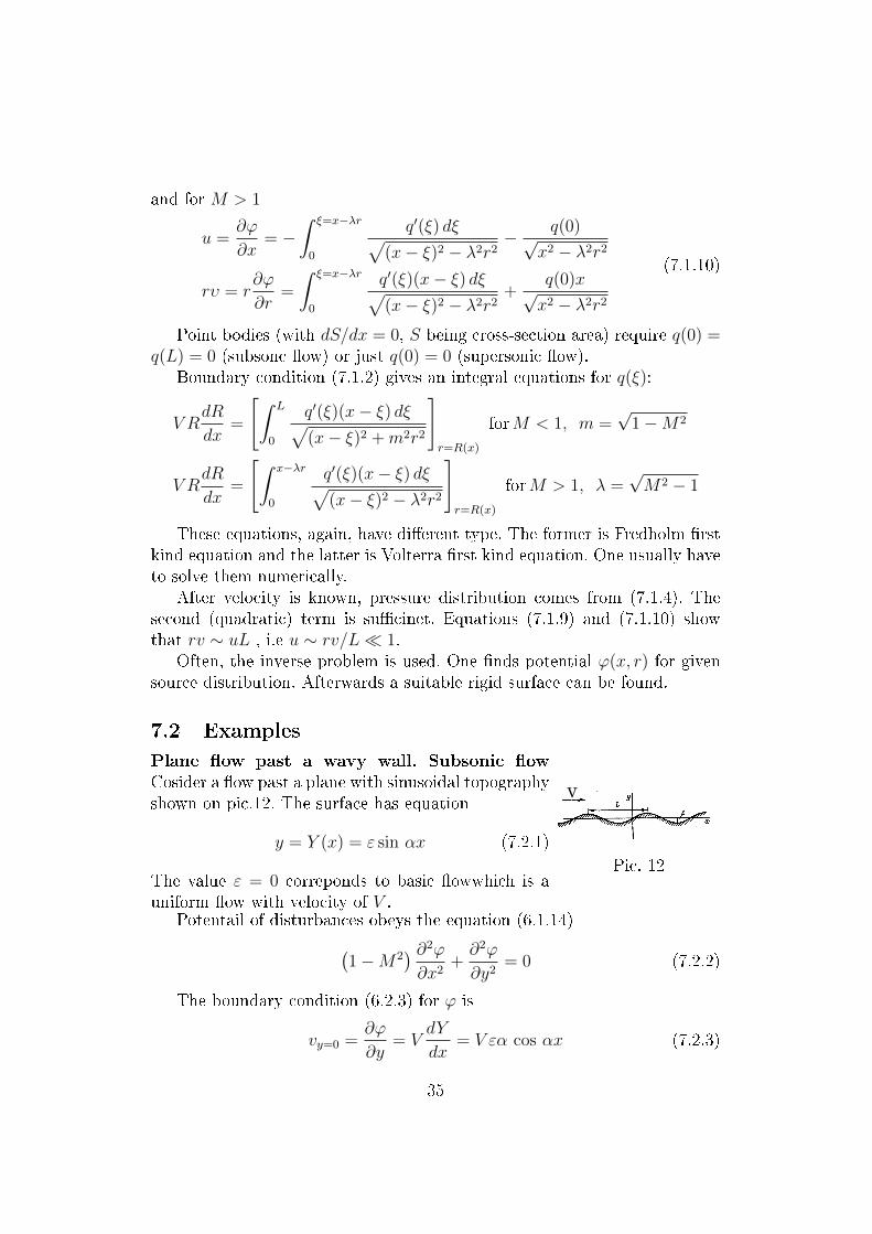
Plane ow past a wavy wall. Subsonic ow
Cosider a ow past a plane with sinusoidal topographyshown on pic.12. The surface has equation
y = Y (x) = ε sin αx (7.2.1)
The value ε = 0 correponds to basic owwhich is auniform ow with velocity of V .
Pic. 12
Potentail of disturbances obeys the equation (6.1.14)(1−M2
) ∂2ϕ
∂x2+∂2ϕ
∂y2= 0 (7.2.2)
The boundary condition (6.2.3) for ϕ is
vy=0 =∂ϕ
∂y= V
dY
dx= V εα cos αx (7.2.3)
35

As the wall is innite, the velocity is bounded at innity u = ∂ϕ/∂xυ = ∂ϕ/∂y at y →∞.
Let M2 < 1. We use Fourier method solving (7.2.2)
ϕ = F (x)G(y)
For F and G we have
F ′′
F=
−G ′′
(1−M2)G= −λ2
Value of λ is real and positive as the solution is periodic on x.Hence
F = A sinλx+B cosλx
G = A1 exp(−√
1−M2λy) +B1 exp(√
1−M2λy)
Boundness at y →∞ requires B1 = 0, and (7.2.3) gives
A = 0, λ = α, −A1B√
1−M2 = V ε
The solution is
ϕ = − V ε√1−M2
exp(−yα√
1−M2) cosαx
Velocity componets and pressure are
u =V εα√1−M2
exp(−yα√
1−M2) sinαx
v = V εα exp(−yα√
1−M2) cosαx
p− p1 = 4p = − ρ1V2εα√
1−M2exp(−yα
√1−M2) sinαx
Disturbances have maximal magnitude at the wall and graually decaygoing from it. It is eqsy to show that drag force is zero.
Linear theory is valid if
u
V 1,
v
V 1,
(γ + 1)M2
|1−M2||u|maxV
1.
For this particular problem it means
εα√1−M2
1,(γ + 1)M2εα
(1−M2)3/2 1
The second condition is stronger and more restricitve for the wall steepnessεα.
36

Plane ow past a wavy wall. Supersonic ow Let M > 1. Generalsolution of (7.2.2) is
ϕ = F (x−√M2 − 1y) +G(x+
√M2 − 1y)
Characteristics of (7.2.2 are straight lines
x−√M2 − 1y = const, x+
√M2 − 1y = const.
Functions F and G are constant at this lines, respectively. As no disturbancescome from innity, G = 0.
Boundary condition at the wall gives
v =∂ϕ
∂y= −√M2 − 1F ′(x) = V
dY
dx= V εα cos αx
and F is
F (x) = − V ε√M2 − 1
sin αx
Hence,
ϕ = − V ε√M2 − 1
sin[α(x−√M2 − 1y
)]u = − V εα√
M2 − 1cos[α(x−√M2 − 1y
)]v = V εα cos
[α(x−√M2 − 1y
)]4p =
ρ1V2εα√
M2 − 1cos[α(x−√M2 − 1y
)]In supersonic ow, disturbances do not decay but keep constant value
along characteristics x−√M2 − 1y = const. Wavy drag force apprears. The
force per period is
X =
∫ l
0
4pdYdx
dx =ρ1V
2
√M2 − 1
∫ l
0
(εα cos αx)2dx
Physically, it means energy tranfer by acoustic waves.
Supersonic ow past a slender cone Consider an axisymmetric supersonicow with small disturbances. Set a linear source distribution q(ξ) = aξ in(7.1.5). Then using (7.1.6), we obtain
ϕ(x, r) = −ax
cosh−1 x
λr−
√1−
(λr
x
)2
37

and velocity components are (7.1.8)
u = −a cosh−1 x
λr
v = aλ
√1−
( xλr
)2
.
This is a conical solution as all functions depend on x/r only. There is acone with x/r = cot δ where boundary condition is satised, i.e. u/v = cot δ.This gives relation between a and δ
a =V δ√
cot2 δ − λ2 + tan δ cosh−1(
cot δλ
)For a slender cone δ 1
a = V δ2
u = −V δ2 ln2
λδ, v = V δ
Cp = 2δ2
(ln 2λδ − 1
2
) (7.2.4)
For plane ows past a wedge, Cp ∼ δ, so pressure on a cone has dierentorder of magnitude.
7.3 Similarity rules
Plane ows Remind the equation for potential Potentail of disturbancesobeys the equation (6.1.14)(
1−M21
) ∂2ϕ
∂x2+∂2ϕ
∂y2= 0 (7.3.1)
The shape of the boundary may be given in the form
y = h1Y(xL
)= τ1LY
(xL
)with non-dimentional thickness τ1 = h1/L, or in comletely non-dimensionalform
y
L= τ1f
(xL
)(7.3.2)
The boundary condition (6.2.3) for ϕ is(∂ϕ
∂y
)y=0
= V1dY
dx= V1τ1Y
′(xL
)(7.3.3)
38

where V1 is the free-stream velocity.The pressure coecient on the boundary is
Cp1 = − 2
V1
(∂ϕ
∂x
)y=0
(7.3.4)
Now consider the pontential Φ(ξ, η) pf a second ow. Let Φ be related toϕ by the relation
ϕ(x, y) = AV1
V2
Φ(ξ, η) = AV1
V2
Φ
(x,
√1−M2
1
1−M22
y
)(7.3.5)
for some constant A. The corrpespondence between coordinate systems is
ξ = x, η =
√1−M2
1
1−M22
y
Introducing (7.3.5) in (7.3.1), we nd the equation for Φ:
(1−M2
2
) ∂2Φ
∂ξ2+∂2Φ
∂η2= 0 (7.3.6)
Hence, Φ describes a ow with Mach number of M2. The boundarycondition (7.3.3) gives(
∂ϕ
∂y
)y=0
= AV1
V2
√1−M2
1
1−M22
(∂Φ
∂η
)y=0
= V1τ1Y′(xL
)(7.3.7)
The only variable in (7.3.7) is x/L. The equations (7.3.7) can be alsowritten as (
∂Φ
∂η
)η=0
= V2τ2Y′(xL
)As Y ′ is the same in both case, we have a relation between A, τ1 and τ2:
A
√1−M2
1
1−M22
τ2 = τ1 (7.3.8)
Using the same function Y means that we consider a family of bodyshapes. They are not geometrically similar but one shape can be obtainedfrome another by proper stratching or compression towards the plane y = 0.
39

The prussure coecients can also be rewrtitten as
Cp1 = − 2
V1
(∂ϕ
∂x
)y=0
= − 2
V2
A
(∂ϕ
∂ξ
)η=0
For the second ow, the pressure coecient is
Cp1 = − 2
V2
(∂ϕ
∂ξ
)η=0
(7.3.9)
Equations (7.3.8) and (7.3.9) set the similarity rules. Two member ofa family of shapes characterized by relative thicknesses τ1 and τ2 have thepressure distributions Cp1 and Cp2. If the Mach numbers of the ows are M1
and M2, respetively, then Cp1 = ACp2 and
τ1 = A
√1−M2
1
1−M22
τ2.
The same can be expressed by formula
CpA
= g
(τ
A√
1−M2
)(7.3.10)
g is a function, the factor A is arbitrary.The crucial point of deriving this similarity rule is linearity of the equation
and boundary conditions. The situation is dierent for transonic ows (nonlinearequations) and axisymmetric ows (nonlinear on the shape function boundaryconditions).
Equation (7.3.10) is a generalization of well known similarity rules.
1. If A = 1, we have Cp = g(τ/√
1−M2).
2. If A = 1/√
1−M2, we have Cp = g(τ)/√
1−M2.
3. If A = τ , we have Cp = τg(√
1−M2).
4. If A = 1/(1−M2), we have Cp = g(τ√
1−M2)/(1−M2).
The rst three methods are dierent form of Prandtl-Glauert rule. Method1 states that Cp remains constant if the thickness follows change of Machnumber in proper way. Method 2 states that for given shape Cp depends onMach number as (1−M2)−1/2, and method 3 states that Cp is proportionalto τ for xed M .
40

Method 4 is a Goethert rule which is not staightforwards for plane owsbut is still valid for axisymmetric ones.
All equations in this subsections were written for subsonic ows, but sinceonly expressions like
√(1−M2
1 )/(1−M22 ) were actually used they are still
valid for supersonic ones with change 1 −M2 to M2 − 1. The invariant onthe type if ow form of equation (7.3.10) is
CpA
= g1
(τ 2
A2(1−M2)
)Axially symmetric ows For axially symmteric ows it is not possibleto state boundary conditions for potential at r = 0 due to singularity.
Equation for potential is (7.1.1)(1−M2
1
) ∂2ϕ
∂x2+∂2ϕ
∂r2+
1
r
∂ϕ
∂r= 0
and the transformation between two ows with potential ϕ(x, r) andΦ(ξ, R)is almost the same as for plane case:
ϕ(x, r) = AV1
V2
Φ(ξ, η) = AV1
V2
Φ
(x,
√1−M2
1
1−M22
r
)(7.3.11)
The analog to (7.3.3) is(∂ϕ
∂r
)body
= V1τ1f′(xL
)f is the shape function. We cannot move to r = 0 and have to use exact form(
∂ϕ
∂r
)r=τ1Lf(x/L)
= V1τ1f′(xL
)Introducing Φ, we have(
∂ϕ
∂r
)r=τ1Lf(x/L)
= AV1
V2
√1−M2
1
1−M22
(∂Φ
∂R
)R=τ1
√1−M2
11−M2
2Lf(x/L)
(7.3.12)
On the other hand, Φ is a solution for the problem with incoming velocityof U2 and the shape function F (R):(
∂Φ
∂R
)R=τ2LF (x/L)
= V2τ2F′(xL
)(7.3.13)
41

In order to compare (7.3.12) and (7.3.12), it is required that the shapefunctions are the same: f(x/L) = F (x/L), which is the same condition asbefore. In addition, it is , that
τ1
√1−M2
1
1−M22
= τ2.
Taking this into account, (7.3.12) gives
τ1f′(xL
)= A
√1−M2
1
1−M22
τ1
√1−M2
1
1−M22
f ′(xL
)This implies the only possible value of A:
A =1−M2
2
1−M21
(7.3.14)
The pressure coecient for axially symmetric ows is
Cp1 = − 2
V1
(∂ϕ
∂x
)r=τ1Lf(x/L)
− 1
V 21
(∂ϕ
∂r
)2
r=τ1Lf(x/L)
Using (7.3.11) we have similar relation in term of Φ:
Cp1 = − 2
V2
(∂Φ
∂ξ
)R=τ1
√1−M2
11−M2
2Lf(x/L)
− A2
V 22
1−M21
1−M22
(∂Φ
∂R
)2
R=τ1
√1−M2
11−M2
2Lf(x/L)
Using (7.3.14), we factor out the constant A and obtain
CpA
= g
(τ
A√
1−M2
)Unlike the case of plane ow, A cannot be chosen arbitrary since it must
satisfy (7.3.14). This value is A = (1−M2)−1. This gives Goehert's similarityrule:
Cp(1−M2) = g(τ√
1−M2) (7.3.15)
Diving both sides by τ 2(1−M2) gives the alternate form
Cpτ 2
= g1(τ√
1−M2) (7.3.16)
There are no free parameters left in this rule, so it could be adjusted tobe valid for transonic ows.
42

8 Hypersonic ows past a blunt body
8.1 Flow past a sphere
Consider a hypersonic ow of perfect gas withheat capacities ratio γ past a sphere of radiusof rb (pic.13). Let the ow far upstream of thesphere be unifrom, its velocity and density beV and ρ0.Assume also M 1. The bow shock in frontof the sphere is strong near the axis of symetryand the gas density after it is close to the limitone and approximately
Pic. 13: Spherical coordinates
ρ =γ + 1
γ − 1ρ0 ≡
ρ0
ε, ε 1
Assume that the shape of the bow shock is close the sphere of radius ofrs.
Spherical coordinates r, θ, ϕ (pic.13) are convenient for this problem. Weuse Gromeka-Lamb equation of motion taking into account uniformity of theincoming ow
curlV ×V = T grad s (8.1.1)
(T is absolute temperature, s is specic entropy).In our coordinates there is only one non-zero component of curlV:
(curlV)ϕ =1
r
(∂rυθ∂r− ∂υr∂ϑ
)(8.1.2)
Hence, left-hand-side of (8.1.1) takes form
curlV ×V =
∣∣∣∣∣∣er eθ eϕ0 0 (rotV)ϕvr vθ 0
∣∣∣∣∣∣ (8.1.3)
Due to axial symmetry there exists streamfunction ψ:
∂ψ
∂r= ρvθr sin θ,
∂ψ
∂θ= −ρvrr2 sin θ (8.1.4)
and
(curlV)ϕ =1
r
[∂rvθ∂r− ∂υr
∂θ
]=
=1
ρr sin θ
∂2ψ
∂r2− 1
ρr3
cos θ
sin θ
∂ψ
∂θ+
1
ρr3 sin θ
∂2ψ
∂θ2
(8.1.5)
43

Projecting (8.1.3) on eθ direction with (8.1.1) gives
vr
(1
ρr sin θ
∂2ψ
∂r2− 1
ρr3
cos θ
sin θ
∂ψ
∂θ+
1
ρr3 sin θ
∂2ψ
∂θ2
)= T
1
r
∂ s
∂ θ(8.1.6)
Thus we transform vector equation of motion (8.1.1) to a scalar one. Now,we transform right-hand-side of (8.1.6) with thermodynamic relation
dh = Tds+dp
ρ
Entropy s depends on ψ only after the shockwave. We can nd withdependence since ψ is continuous. In the incoming ow
ψs =1
2ρ0V r
2s sin2 θ (8.1.7)
Denote m = ρ0V cos θ local mass ux and consider Hugoniot adiabat:
m2 = p−p11/ρ0−1/ρ
(8.1.8)
γγ−1
(pρ− p0
ρ0
)− p−p0
2
(1ρ
+ 1ρ0
)= 0 (8.1.9)
Equations (8.1.8),(8.1.9) gives expressions for dp, dh along the shock wave
dp = 2mdm (1/ρ0 − 1/ρ) = −2ρ20V
2 sin θ cos θ (1/ρ0 − 1/ρ) dθ
dh =1
2dp
(1
ρ+
1
ρ0
)T ds =
1
2dp
(1
ρ+
1
ρ0
)− dp
ρ=
= ρ21V
2 sin θ cos θ (1/ρ1 − 1/ρ)2 dθ = −V 2 sin θ cos θ(1− ε)2dθ
(8.1.10)
Hence, we can put factor of ψθ ∼ vr explicitly to the right-hand-side of(8.1.6):
T1
r
∂ s
∂ ϑ= T
1
r
ds
dψ
∂ ψ
∂ ϑ(8.1.11)
Equation (8.1.10) gives values of sθ and φθ right after the shock wavesand allows deriving of sψ:
Tds
dϑ
∣∣∣∣s
= Tds
dψ
∂ ψ
∂ ϑ
∣∣∣∣s
= −ρ0V2 sin θ cos θ(1− ε)2
and
Tds
dψ= −V (1− ε)2
ρ0r2s
(8.1.12)
44

Finally, equations (8.1.4), (8.1.6), (8.1.11),(8.1.12) give equation for ψ
ψrr +sin θ
r2
∂
∂θ
(ψθ
sin θ
)=V r2(1− ε)2 sin2 θρ1
r2sε
2(8.1.13)
Boundary conditions for (8.1.13) are continuity of ψ at the shock wave(8.1.7) and tangential velocity vθ = V sin θ at r = rs.
Equation (8.1.13) has a solution of ψ = f(r) sin2 θ, with f(r) satisfyingODE
f ′′ − 2
r2f =
ρV r2(1− ε)2
ε2r2s
Introducing ξ = r/rs and g = f/(ρ0V r2s) we obtain Euler equation for
g(ξ)
ξ2g′′ − 2g =(1− ε)2
ε2ξ4 g(1) =
1
2g′(1) =
1
ε
The solution is
g =1
3
(1
2− 5A+
1
ε
)ξ +
1
3
(1 + 2A− 1
ε
)1
ξ+ Aξ4 A =
(1− ε)2
10ε2
The position of the sphere corresponds to g = 0. At ξ = 1 values of g, g′,and g′′ are known and for ξ = 1 + εη we have
g =1
2+ η +
1
2η2
which gives ηb = −1. Returning to physical coordinates results rs − rb =εrs.
8.2 Basic ideas of Cherny method
For an arbitrary blunt body, there is a thin shock layer between the shockwave and the body surface. If the ow is hypersonic, the density in this layerρ is much greater than the density in the incoming ow ρ1. The ration ofthese densities ε = (γ − 1)/(γ + 1) is small and we can expand all unknownfunction onto series of ε
45

Let the body surface is y = y(x), where xis arclength from the axis of symmetry alongthe tangential surface t, and y is the distanceMN from a given pointM to the surafce alongthe normal (14). Let α be the angle betweentangent to t and the axis of symmetry, anddistances from points N and M are lt and l.Let us assume that the radius of curvature ofthe body surface R obeys |dR/dx| 1. Thestreamfunction ψ for these coordinates is
dψ = ρuldy − ρvl(1 + y/R)dxPic. 14: Curvilinearcoordinates
where u and v are velocity componets along x, y.As the shock layer is thin, pressure change along x coordinate is much
greater than along y. Equation of motion and adiabatic law give
ρu∂u
∂x+ ρv
∂u
∂y+∂p
∂x= 0
1
1 + y/R
∂v
∂x− u
R + y= −l ∂p
∂ψ;
∂
∂x
(p
ργ
)= 0
(8.2.1)
Boundary conditions at the shock wave are
p =2
γ + 1ρ1V
21 sin2 β − γ − 1
γ + 1p1
ρ1
ρ=γ − 1
γ + 1+
2
γ + 1
1
M21 sin2 β
=
=
(uy ′
1 + y/R− v)V1
(cosα− sinα
y′
1 + y/R
)[V1
(sinα + cosα
y′
1 + y/R
)]−1
=
= u+vy ′
1 + y/R(8.2.2)
where M1 is Mach number in the incoming ow and β is an angle betweentangent to shock wave and the axis of symmetry.
We seek for a solution of (8.2.1) with boundary conditions (8.2.2) in theform
u = u(0) + εu(1) + . . . ; v = εv(0) + . . .
p = p(0) + εp(1) + . . . ; ρ =ρ(0)
ε+ ρ(1) + . . .
(8.2.3)
46

The rst approximation gives pressure distribution
p(0) = ρ1V2
1 sin2 α(x)− 1
Rlt
∫ ψ∗
ψ
u(0)dψ, ψ∗ =1
2ρ1V1l
2t
Higher order term in (8.2.3) allows nding the thickness of the shocklayer.
47

9 Weak shock wave structure
Gas dynamics usually deals with ideal gas with zero heat conductance. Flowsof such medium are isentropic as there are no physical mechanisms for theentropy production. Exceptions usually involve external heat sources or sinks.As a consequence, Euler equations for non-stationary ows are hyperbolic andadmit shock waves. These shocks are treated as innitely thin surface whereparameters of the ow change. On the other hand this means that spatialderivatives of those functions are quite large and dissipative process (viscosityand heat conductance) which are proportional to velocity and temperaturegradients cannot be neglected. In this section, we take these processes intoaccount and consider the inner structure of a shock wave.
Consider a steady one dimensional ow of a compressible viscous (η isdynamic viscosity coecient) heat-conductive (κ is heat conductance) gas.
Governing equations areddx
(ρu) = 0ddx
(p+ ρu− 4
3η dudx
)= 0
ρudSdx
= 43η(dudx
)2+ d
dx
(κ dTdx
) (9.0.4)
We assume that the second (volume) viscosity coecient is zero. This assumptionis good enough for monoatomic gases and other media when the ow relaxationtime is much large than the internal degrees of freedom relaxation time.
The second thermodynamic law TdS = dh−dp/ρ and mass and momentumconservation laws allow rewriting of the entropy equation:
d
dx
[ρu
(h+
u2
2
)− 4
3ηudu
dx− κ
dT
dx
]= 0 (9.0.5)
We state boundary conditions for these equations at−∞ and +∞ requiringall parameters ρ, u, p, T be constant. We denote these constants by subindeces0 and 1, respectively.
First two equations of (9.0.4) and (9.0.5) admit rst integrals:
ρu = ρ0u0 (9.0.6)
p+ ρu2 − 4
3ηdu
dx= p0 + ρ0u
20 (9.0.7)
ρu
(h+
u2
2
)− 4
3ηudu
dx− κ
dT
dx= ρ0u0
(h(0) +
u20
2
)(9.0.8)
Considering left-hand-sides at +∞ with zero derivatives, we obtain Rankine-Hugoniot conditions.
Discontinuity is no longer possible, as it means innite value of derivativedu/dx which contradict to (9.0.7). Further we will consider heat conductanceand viscosity separately.
48

9.1 Inviscid heat conductive gas
In this case (9.0.7) is algebraic equation:
p+ ρu2 = p0 + ρ0u20
together with (9.0.6) it describes all intermediate states:
p = p0 + ρ0u20
(1− V
V0
), V = 1/ρ. (9.1.1)
At the p, V plane, this equation describes all points on a straight linesegment AB which connects initial ("0 point A) and terminal ("1 point B)states at Higoniot adiabat (pic.??). A bit to the left from point A this lineis above the Poisson adiabat going through A, the same is valid for points abit to the right from B. Hence, there is a Poisson adiabat which is tangentto AB. This adiabat corresponds to the maximal value of entropy Smax. Wecan nd using the condition of tangent.
As the shock wave is weak S1 − S0 is of order of (p1 − p0)3 or (V1 − V0)3.We see that on the segment AB entropy can be larger than S1 and S0, soS − S0 can be large than S1 − S0. That is why we keep the term S − S0
together with (V − V0)2 in the expansion of p− p0 in a small vicinity of A
p− p0 =
(∂p
∂V
)S0
(V − V0) +1
2
(∂2p
∂V 2
)S0
(V − V0)2 +
(∂p
∂S
)V0
(S − S0)
The equation of AB is
p−p0 =p1 − p0
V1 − V0
(V −V0) =
(∂p
∂V
)S0
(V −V0)+1
2
(∂2p
∂V 2
)S0
(V1−V0)(V −V0)
We nd the tangent point: it corresponds to V − V0 = 1/2(V1 − V0). Themaximal entropy can be easily found:
Smax − S0 =1
8
(∂2p/∂V 2)S0(∂p/∂S)V0
(V1 − V0)2.
Maximal entropy change in a weak shock wave is a second-order smallvalues. The entropy rst rises to its maximal value and then goes down tomake the total entropy change be third-order small value. The existence ofan extremum of entropy implies the presence of an inection point on thetemperature prole. Indeed, without viscosity, the entropy equation reads
ρuTdS
dx= κ
d2T
dx2(9.1.2)
49

We are now able to estimate thickness of the shockwave. We divide bothparts of (9.1.2) by T and integrate over x (we take into account that ρu isconstant):
ρ0u0(S − S0) = κx∫
−∞
1
T
d2T
dx2dx = κ
1
T
dT
dx+
T∫T0
dT
dx
1
T 2dT
. (9.1.3)
For large enough x, we have dT/dx = 0 the rst term in brackets vanishesand we have
ρ0u0(S − S0) = κT∫
T0
dT
dx
1
T 2dT.
We dene the shock wave thickness ∆x for the presence of heat conductanceonly as
T1 − T0
∆x=
∣∣∣∣dTdx∣∣∣∣max
. (9.1.4)
Simple estimation gives
ρ0u0(S − S0) = κ(T1 − T0)2
dx
1
T 20
dT.
We can replace temperature jump by pressure change:
T1 − T0 =
(∂T
∂p
)S
(p1 − p0) =V0
cp(p1 − p0).
Here we used the second thermodynamics law formulation: cpdT = Tds+pdV .
In a weak shock wave the entropy change is
T0(S1 − S0) =1
12
(∂2V
∂p2
)S
(p1 − p0)3
Using approximate relations: ∂2V ∂p2 ∼ V0/p20, κ ∼ ρ0cplc0, c0 ∼ u0,
p0 ∼ cpρ0T0 for mean free path length l, mean chaotic velocity c0, we obtain
∆x ∼ lp0
p1 − p0
From (9.1.3), we see that maximal local entropy change Smax − S0 isproportional to ∆T/∆x ∼ (∆p)2 while terminal entropy change is one orderof magnitude less.
In this solution we see that only temperature must be continuous, whileall other functions (velcoity, density, pressure) may have discontinuity.
50

9.2 Viscous non heat conductive gas
Now consider the case κ = 0, η > 0. The entropy equation is
ρudS
dx=
4
3η
(du
dx
)2
so entropy grows monotonically. The line AB on pV plane is below adiabatgoing through the point B. The equation of the AB line is
p = p0 + ρ0u20
(1− V
V0
)+
4
3ηdu
dx(9.2.1)
As this line is below the straight line AB du/dx < 0 inside the shock wave.We dene the shock wave thickness as∣∣∣∣u1 − u0
∆x
∣∣∣∣ =
∣∣∣∣dudx∣∣∣∣max
.
Maximal value of the derivative corresponds to maximal vertical distancebetween the straight line AB and actual path (9.2.1). Taking a point in themiddle between A and B, we estimate
4
3ηdu
dx=
1
8
(∂2p
∂V 2
)SA
(V1 − V0)2
The velocity change is
u0 − u1 = −√
(p1 − p0)(V0 − V1) =
√(p1 − p0)2
∣∣∣∣∂V∂p∣∣∣∣ ∼ p1 − p0
p0
c0
and viscosity η ∼ ρ0lc0. The shock wave thickness is
∆x = lp0
p1 − p0
The viscous solution give continuous solution for all functions. This meansthat friction is a principal mechanism of transferring kinetic energy of thegas into its heat energy.
Considering non-weak shock waves, one may obtain its thickness less thanmean free path, which is physically meaningless. The solution of this paradoxis that transport coecients cannot be constant throughout the whole rangeof temperatures and this fact must be taken into account. For strong wavesthe solution must be based on kinetics theory and consider possible excitationof internal degrees of freedom.
51

10 Thermally non-equilibrium ows
10.1 Relaxation to equilibrium
The only way of information transport in gas is collisions between its molecules.Hence there is a reference time scale which is dened by time betweencollision. It is
τcoll =l
c0
=1
nc0σ,
where l is mean free path, c0 mean velocity of chaotic motion, n is numberconcentration and σ is collision cross-section. For air at normal conditionsl 10−8 m and τcol ∼ 10−10 s. This time is usually much less than referencetime of a gas dynamics problem, so we can assume that collisions take placevery often.
On the other hand, there could be situations when one collision is notenough for molecules to exchange energy. This situations occur if quantumeects are sucient. For diatomic gases two main quantum features maybe observed, they connected to internal rotations and oscillations in themolecules.
Energy of the internal rotation is proportional to the moment of inertiaand allowed by quantummechanics angular velocities. The reference temperatureTr = Erot/k for most gases is lower or around 10 K with the exception forH2 and D2, these gases have reference rotation temperature around 80 K.Anyway, for room temperature or above gases are in far classical diapasonand the energy got of lost by a molecule during a collision is enough toexcite or deactivate rotational degrees of freedom. Experiments show thatthe rotational energy comes to its equilibrium value after about 10 collisionsfor air gases and 150 300 collisions for hydrogen and deuterium. This givesan estimation for a relaxation time.
Sometimes, the relaxation to equilibrium takes much longer. Considerthis process in details. Let N be a number of molecules which are excited orcome to a new state due to chemical reaction, Ne be an equilibrium numberof such molecules. In general, there is a law:
dN
dt= f(N, T, ρ, . . . )
but for small values of relative dierence |N − Ne|/Ne 1 one can expandthis law into Taylor series and obtain
dN
dt=Ne −N
τ
52

with a solution
N = N0 exp
(− tτ
)+Ne
[1− exp
(− tτ
)]The value of τ is relaxation time.If there are several processes with quite dierent relaxation times one
observes series of relaxation according to their timescales.For a gas dynamics problem, there is another reference time τf . For each
process with relaxation time τ there are three possibilities:
• τ τf quasi-equilibrium ow
• τ ∼ τf nonequilibrium ow
• τ τf frozen ow
In the latter case one can assume that there is no relaxation at all, andthe state of non-equilibrium degrees of freedom does not change.
10.2 Sound propagation in a gas with relaxation
Consider small perturbation of the rest state for a gas with relaxation.Let the energy of internal oscillations be the relaxing value. We introduceto temperatures: T corresponding to translational and rotational degreesof freedom and vibrational corresponding to the current level of energy ofvibrations. Assume the the gas is perfect with constant heat capacities.
The governing equations are:
dρdt
+ ρ∇ · ~v = 0, d~vdt
+ 1ρ∇p dh
dt− 1
ρdpdt
= 0
h = cpT + ev(Tv) p = ρRT devdt
= ev(T )−ev(Tv)τ
(10.2.1)
Excluding h from the third equation (10.2.1) we obtain
dp
dt− a2
v
dρ
dt+ ρ(γ − 1)
evdt
= 0. (10.2.2)
Here γ stands for heat capacities ratio for a gas with frozen degree of freedom,hence af is called frozen speed of sound.
Consider small perturbations of a uniform state (denoted by primes):
~v = ~v′, p = p0 + p′, ρ = ρ0 + ρ′, T = T0 + T ′, Tv = T0 + T ′v (10.2.3)
53

As these perturbations are small with their derivatives, nonlinear termcan be neglected after substitution (10.2.3) to (10.2.1), (10.2.2):
∂ρ′
∂t+ ρ0∇ · ~v′ = 0,
∂~v′
∂t+
1
ρ0
∇p′ = 0
∂p′
∂t− a2
f
∂ρ′
∂t+ ρ0(γ − 1)ev
∂T ′v∂t
= 0∂Tv∂t
=T ′ − T ′vτ0
T ′
T0
=p′
p0
− ρ′
ρ0
devdt
=devdTv
∣∣∣∣Tv=T0
(10.2.4)
The second equation implies the existence of velocity potential, so introducingϕ:
~v′ = ∇ϕ
from two rst equations (10.2.4) we have
∂ρ′
∂t+ ρ0∆ϕ = 0, p′ = −ρ0
∂ϕ
∂t(10.2.5)
Exclude T ′ from the last equation:
∂Tv∂t
=1
τ0
(T0
p0
p′ − T0
rho0
ρ′ − T ′v)
Taking time derivative of this equation and the third equation (10.2.4 weget
∂2p′
∂t2− a2
f
∂2ρ′
∂t2+ ρ0(γ − 1)ev
∂2T ′v∂t2
= 0
∂2Tv∂t2
=1
τ0
(T0
p0
∂p′
∂t− T0
rho0
∂ρ′
∂t− ∂T ′v
∂t
) (10.2.6)
exclude T ′v:
∂2p′
∂t2− a2
f
∂2ρ′
∂t2+
1
τ
[(λT0
p0
+ 1
)∂p′
∂t−(λT0
ρ0
+ a2f
)∂ρ′
∂t
]= 0
where λ = ρ0(γ − 1)ev, and nally obtain the equation for potential
∂
∂t
(∂2ϕ
∂t2− a2
f∆ϕ
)+
1
τ
(∂2ϕ
∂t2− a2
e∆ϕ
)= 0. (10.2.7)
We use
τ = τ0
(λT0
p0
+ 1
)−1
, a2e =
(λT0
ρ0
+ a2f
)(λT0
p0
+ 1
)−1
.
54

We simplify these expressions
τ = τ0
(λT0
p0
+ 1
)−1
=τ0p0
ρ0(γ − 1)evT0 + p0
=τ0cvev + cv
= τ0cvcve
using cve constant volume heat capacity for equilibrium state, and
a2e =
λT0 + a2fρ0
λT0 + p0
p0
ρ0
=ρ0(γ − 1)evT0 + γp0
ρ0(γ − 1)evT0 + p0
p0
ρ0
= fraccp + evcv + evp0
ρ0
= γep0
ρ0
.
We see that ae has the same structure as af but it involves heat capacitiesration for the equilibrium state. If is clear that γe < γ, so ae < af .
The equation for small disturbances propagation (10.2.7) involves twowave operators with dierent speed of sound. Let us investigate its limitcases.
If τ → ∞ we have a frozen ow and (10.2.7) takes form of usual waveequation with classical (frozen) speed of sound:
∂2ϕ
∂t2− a2
f∆ϕ = 0,
provided initial conditions satises this equation.It the relaxation time τ is small, we have
∂2ϕ
∂t2− a2
e∆ϕ = 0,
so disturbances propagate at equilibrium speed of sound.
10.3 Dispersion relation
Consider one dimensional (plane) disturbances. The governing equation (10.2.7)reads
∂
∂t
(∂2ϕ
∂t2− a2
f
∂2ϕ
∂x2
)+
1
τ
(∂2ϕ
∂t2− a2
e
∂2ϕ
∂x2
)= 0. (10.3.1)
For monochromatic plane wave
ϕ = A exp [i(kx− ωt] (10.3.2)
it gives dispersion relation
−iω(−ω2 + a2fk
2) +1
τ(−ω2 + a2
ek2) = 0,
55

which is relation between wavenumber and frequency:
k = ω
√1− iωτ
a2e − iωτa2
f
. (10.3.3)
The wavenumber is now complex and k = kr + iki, so the disturbance(10.3.2) is rewritten
ϕ = A exp(−kix) exp
[ikr
(x− ω
krt
)]the ratio ω
kris phase velocity and the exponent with real argument −kix
stands for growth for negative ki and decay for ki.Consider dierent asymptotic case. Let ωτ 1. Neglecting terms of order
of (ωτ)2, we obtain
k =ω
ae+ i
ω
ae
ωτ
2a2e
(a2f − a2
e).
Phase velocity for these waves if equilibrium speed of sound. The imaginarypart is positive so disturbances decay and decay rate is proportional to af −ae > 0.
For short (high-frequency waves)
k =ω
af+ i
1
2τa3f
(a2f − a2
e).
For general case the equation (10.3.3) gives
kr = mω cos θ ki = mω sin θ
m =(
1+(ωτ)2
a4e+(ωτ)2a4f
)1/4
, 2θ = atanωτ(a2f−a
2e)
a2e+(ωτ)2a2f.
The decay rate has maximum at ωτ = ae/af . Typical dependence of phasevelocity ω/kr and decay rate ki/ω on normalized frequency ωτ is shown atthe picture 15.
Pic. 15: Phase velocity and decay rate of disturbances in gas with relaxation
56

10.4 Flow in a de Laval nozzle
Consider a ow in a de Laval nozzle. For stationary one dimensional owtemperature depends on Mach number as
T0
T= 1 +
γ + 1
2M2
If a hypersonic ow (M > 10) is present at the exit of the nozzle,temperature drops by factor of 40 at the nozzle length. Assuming roomtemperature near the exit, it is clear that there is very high temperature inthe stagnation region, and vibrational degrees of freedom are excited there.Going downstream temperature goes down and these degrees of freedomget deactivated. The energy of molecules or any other thermodynamicalparameter corresponding to vibrational degrees of freedom obeys relaxationequation
dq
dt=qe(ρ, T )− q
τ(10.4.1)
for a state parameter q, thermodynamical parameters ρ, T , and relaxationtime τ(ρ, T ).In a nozzle, the ow is one-dimensional and stationary, so d/dt = ud/dx,thermodynamical parameters ρ, T are given function of x. Consider somesimple solutions.
1. Let qe = const, τ = const. The solution of (10.4.1) is
q = qe + (q0 + qe)e−t/τ
Considering initial condition q0 = qe, we have equilibrium ow in the wholenozzle
2 qe = qe(t) is a given function, τ = const. In this case the equation (10.4.1)has a solution
q =1
τe−t/τ
t∫0
eξ/τqe(ξ)dξ + q0e−t/τ
Integrating by parts (n+ 1) times, we obtain
q =n∑i=0
(−1)iτ iq(i)e (t)−
[n∑i=0
(−1)iτ iq(i)e (0)
]e−t/τ+(−1)n+1τne−t/tau
t∫0
eξ/τq(n+1)e (ξ)dξ+q0e
−t/τ
57

Assume, there is an equilibrium in the stagnation region. For n = 2 we have
q = qe(t)−τq′e(t)+τ 2q′′e−[−τq′e(0) + τ 2q′′e (0)
]e−t/τ−τ 2e−t/τ
t∫0
eξ/tauqe(3)dξ+q0e−t/τ
or, if the third derivative is small enough
q = qe(t)
[1− τ q
′e(t)
qe(t)+ τ 2 q
′′e (t)
qe(t)
]+ A(t)e−t/τ (10.4.2)
with a bounded function A(t). The reason for non-equilibrium stateappearance in the nozzle is a variation of equilibrium along the nozzle.The reference time of change of qe is
τvar =
∣∣∣∣q′e(t)qe(t)
∣∣∣∣−1
It is the third refence time along with relaxation time τ and the ow refencetime τf = l/u∗, where l is a refernce length and u∗ is reference velocity, e.g.critical speed of sound. The scale τvar only changes along the nozzle, so weconsider its local value in dierent regions.The governing equation (10.4.1) in non-dimensional form is
dq
dt=qe(t)− qτ/τf
There are four dierent cases conserning relation between these scales.
1. τ/τf 1 leads to dq/dt ≈ 0 and q is almost constant. This is almostfrozen ow
2. τ/τf 1 implies q ≈ qe(t), so the ow is almost equilimrium.
3. τ/τvar. In this case (10.4.2) gives q ≈ qe(t), so the ow is almost
equilimrium.
4. τ ∼ τf ∼ τvar. No simplication is possible and the ow in non-equilibrium.
We assumed that there is an equilibrium at the stagnation region, so in theconvergent part of the nozzle it is likely that τ/τvar 1 and the ow isalmost equilibrium.
58

Further downstream, the velocity of the gas increases and its pressuregoes down, so the relaxation time increases. In some region the have non-equilibrium ow as
τ ∼ τf ∼ τvar
Near the exit area, gas is usually rareed, the velocity alomost reaches itsterminal value, pressure and temperature are quite low. This means that τfhas its maximum and the relation τf ∼ τvar. On the other hand, due to lowpressure the relaxation time is small, so
τ
τf 1
and the ow is alomost frozen.One can assume that the middle region is short and neglect changes in thisregion. In this case there are only equilibrium and frozen ows with a sharpborder between them. That is why this method is referred to as 'suddenfrrezing method'.The same procedure can be also applied for a gas jet expansion to vacuum,e.g. from a sonic nozzle. In this case 'sudden freeze' means tranfer fromcontinuum ow to free molecular one.
59

11 Basics of nucleation theory
The considered above non-equilibruim eects involve a pair of molecules andthe equilibruim state of a molecule can be reached during one collision. Inthis section we consider dierent process.
11.1 Energy barrier
During isentropic expansion in a nozzle, temperature and presuure of a gasboth go down and pressure is power function of temperature. If temperatureis low enough, the pressure becomes higher than saturated vapor presuurefor this temperature. This means that the gas (vapor) becomes metastableand pahse transition to liquid (condensation) is possible.The driven force for phase transition is chemical potentials dierence:
∆µ = µv(pv, T )− µl(pv, T ) > 0.
If a particle goes from vapor phase to a liquid one, the free energy decreases.For saturation conditions p = psat, the pahase are at equilibrium and chenicalpotential dierence is zero.One can extimate the chemical potential dierence:
∆µ = [µv(pv, T )− µ(psat, T )] + [µ(psat, T )− µl(pv, T )]
The second term describes the chemical potential variation in liquid whichis much less than the one for vapor. For thermodynamics, one obtains
∆µ = kT lnS, S =pv
psat(11.1.1)
introducing supersaturation S.This equation gives the enegry dierence between a particle in bulk vaporand liquid phase. On the other hand, liquid forms clusters with large amountof molecules and thess clusters have a free surface. The formation of surfacerequires some energy which can be desribed by surface tension coecient γ.Finally, the energy change for n-cluster formation from n vapor molecules is
∆G = −nkT lnS + γA(n)
where the surface area A(n) = 4πr2n and the radius of the cluster rn is
rn = r1n1/3, r1 =
(3v1
4π
)1/3
60

The surface area is
A(n) = s1n2/3 s1 = (36π)1/3
(v1)2/3
Hence,
β∆G = −n lnS + θn2/3, β =1
kT, θ =
γs1
kT(11.1.2)
This function has its maximum at
nc =
(2
3
θ
lnS
]3
.
The cluster with nc molecules is called a critical cluster, maximum of thefunction ∆G∗ = ∆G(nc) represents an energy barrier which a system has toovercome to turn to a new (liquid) state. Droplets which are smaller than ncdissociate on average, while large droplets (> nc) on average grow.In our approxiamtion about surface energy we obtain classical energy barrier
∆G∗ =1
3γA(nc) =
16π
3
(v1)2γ3
(kT lnS)2
or in non-dimensional form
β∆G∗ =4
27
θ3
ln2 S
11.2 Kinetics of nucleation
The equilibrium cluster distribution
ρe(n) = ρ1 exp [−β∆G(n)]
gives large values for large values of n where the bulk term in ∆G dominates,so this distribution diverges. Hence, the actual distribution is aected byinitial conditions and is non-equilibrium.The classical nucleation theory (CNT) uses the following assumptions:
• the elementary process which changes the size of a nucleus is theattachment to it or loss by it of one molecule
• if a monomer collides a cluster it sticks to it with probability unity
• there is no correlation between successive events that change thenumber of particles in a cluster (nucleation is a Markov process)
61

Let fn be a forwrd rate of attachment of a molecule to an n-cluster(condensation) as a result of which it becomes an (n + 1)-cluster, and bnbe a backward rate corresponding to loss of a molecule by an n-cluster(evaporation) as a result of which it becomes and (n1)-cluster. Then thekinetics of the nucleation process is described by the set of coupled rateequations
∂ρ(n)
∂t= fn−1ρ(n− 1, t)− bnρ(n, t)− fnρ(n, t) + bn+1ρ(n+ 1, t)
A net rate at which n-clusters become n+ 1 - clusters is
J(n, t) = fnρ(n, t)− bn+1ρ(n+ 1, t) (11.2.1)
so∂rho(n, t)
∂t= J(n− 1, t)− J(n, t) (11.2.2)
This equiation is called Becker Doring equation.The coecients fn and bn are dened independently. The former one isdetermined by collision frequency nu per unit area:
fn = νA(n), ν =pv√
2πm1kT
where m1 is a mass of one molecule.The backward (evaporation) rate b(n), at which a cluster looses molecules,a priori is not known. It is feasible to assume that this quantity is to alarge extent determined by the surface area of the cluster rather than bythe properties of the surrounding vapor. Therefore bn can be assumed to beindependent on the actual vapor pressure. In order to nd it CNT uses thedetailed balance condition at a so called constrained equilibrium state, whichwould exist for a vapor at the same temperature T and the supersaturationS > 1 as the vapor in question. In the constrained equilibrium the net uxis absent J(n, t) = 0 since it corresponds to the stage before the nucleationprocess starts, and the cluster distribution is given by e(n). From (11.2.1)this implies
bn+1 = f(n)ρe(n)
ρe(n+ 1)
and (11.2.1 gives
J(n, t)1
f(n)ρe(n)=ρ(n, t)
ρe(n)− ρ(n+ 1, t)
ρe(n+ 1)(11.2.3)
62

Assume the nuceation is steady-state, so non-equilibrium concentraions donot depend on time. Hence:
J(n, t) = J,∀n
Taking sum of (11.2.3) for n from 1 to some large number N gives
JN∑n=1
[1
f(n)ρe(n)
]=ρ(1, t)
ρe(1)− ρ(N + 1, t)
ρe(N + 1)
The rst term in right-hand-side is 1 and the second one vanishes as N →∞.Finally, we get
J =
[∞∑n=1
1
f(n)ρe(n)
]−1
Assume, nc 1 as it is required by assumption of spherical clusters. In thiscase the sum can be replacd by an integral:
J =
∞∫n=1
dn
f(n)ρe(n)
−1
The main contribution to the integral comes from n around critical clustersize. In the vicinity of nc
ρe ≈ ρe(n) exp
[−1
2
1
kT∆G′′(nc)(n− nc)2
], ∆G′′(nc) < 0
The Gaussian intergation gives
J = Zfncρe(nc) Z =
√− 1
2π
1
kT∆G′′(nc)
where Z is called Zeldovich factor.Taking into account energy barrier (11.2.2), Zeldovich factor takes the form
Z =1
3
√θ
πn−2/3c
or
Z =
√γ
kT
1
2πρ1r2c
Summarizing, the main result of the CNT states that the steady statenucleation rate is an exponential function of the energy barrier. It works wellfor large enough critical cluster size, which requires small supersaturation.Nozzle ows can shown τf at the region with supersaturation much smallerthan the reference time of nucleation. This leads to high supersaturations(∼ 101 or larger) and CNT is not valid.
63

Ëèíåéíàÿ òåîðèÿ óñòîé÷èâîñòè
ôðîíòîâ ãîðåíèÿ
Ïîñòàíîâêà çàäà÷è îá óñòîé÷èâîñòè ôðîíòîâ ãîðåíèÿ
Èññëåäîâàíèå óñòîé÷èâîñòè â ëèíåéíîì ïðèáëèæåíèè ïðîâîäèòñÿ ïóòåìëèíåàðèçàöèè ãèäðîäèíàìè÷åñêèõ óðàâíåíèé ñ ó÷åòîì ãðàíè÷íûõ óñëî-âèé íà ïîâåðõíîñòè ðàçðûâà. öåëÿõ ïðîñòîòû îãðàíè÷èìñÿ ðàññìîòðåíèåì ñëó÷àÿ, êîãäà òå÷åíèå ïå-ðåä ôðîíòîì è çà íèì ìîæíî ñ÷èòàòü íåñæèìàåìûì .Ïóñòü íåâîçìóùåííûé ôðîíò íàõîäèòñÿ â ïëîñêîñòè x = 0 . Ñêîðîñòüu01 ãîðþ÷åé ñìåñè, çàíèìàþùåé ïîëóïðîñòðàíñòâî x < 0, íàïðàâëåíàâ ïîëîæèòåëüíóþ ñòîðîíó îñè x. Çà ðàçðûâîì ñêîðîñòü u02 = λu01 (ïðèìåäëåííîì ãîðåíèè λ > 1 ). Ïëîòíîñòü ρ01 ïåðåä ôðîíòîì â λ ðàç áîëüøåïëîòíîñòè ρ02 ïîçàäè íåãî, òàê ÷òî ρ01 = λρ02 .Ðàññìîòðèì îòêëîíåíèÿ ïîâåðõíîñòè ôðîíòà îò ïëîñêîé. Òîãäà àáñöèññàïðîèçâîëüíîé òî÷êè ïîâåðõíîñòè ôðîíòà ζ ìîæåò áûòü çàïèñàíà â âèäåôóíêöèè îò y è t , òî åñòü ζ = ζ(y, t) .Ñîîòâåñòâóþùèå èñêðèâëåíèþ ôðîíòà âîçìóùåíèÿ ãèäðîäèíàìè÷åñêèõïàðàìåòðîâ áóäóò òàêæå ÿâëÿòüñÿ ôóíêöèÿìè x, y è t. Ñëåäîâàòåëüíî,âîçíèêàåò íåîäíîìåðíîå íåñòàöèîíàðíîå òå÷åíèå. íåîäíîìåðíîì ñëó÷àå äàâëåíèå p1 è êîìïîíåíòû ñêîðîñòè u1, υ1 ïåðåäôðîíòîì ñâÿçàíû ñî çíà÷åíèÿìè ýòèõ æå ôóíêöèé çà ôðîíòîì p2, u2, υ2
ñîîòíîøåíèÿìè
− ρ01U1(u2 − u1) = (p2 − p1)
[1 +
(∂ζ
∂y
)2]−1/2
,
− ρ01U1(υ2 − υ1) = −(p2 − p1)∂ζ
∂y
[1 +
(∂ζ
∂y
)2]−1/2
,
∂ζ
∂t
[1 +
(∂ζ
∂y
)2]−1/2
=
(u1 − υ1
∂ζ
∂y
)[1 +
(∂ζ
∂y
)2]−1/2
− U1 ,
∂ζ
∂t
[1 +
(∂ζ
∂y
)2]−1/2
=
(u2 − υ2
∂ζ
∂y
)[1 +
(∂ζ
∂y
)2]−1/2
− U2 ,
ρ01U1 = ρ02U2 = const (4)
Çäåñü U1 è U2 åñòü ïðîåêöèè ñêîðîñòåé ãàçà îòíîñèòåëüíî ôðîíòà íàíîðìàëü ê íåìó. Ïåðâûå äâà èç ñîîòíîøåíèé (4) âûðàæàþò çàêîí íåïðå-ðûâíîñòè ïîòîêà èìïóëüñà ïðè ïåðåõîäå ÷åðåç ðàçðûâ ñ ó÷åòîì òîãî, ÷òîâ ñèñòåìå êîîðäèíàò x, y ïîâåðõíîñòü ôðîíòà íå ÿâëÿåòñÿ íåïîäâèæíîé.Äâà äðóãèõ ñîîòíîøåíèÿ - êèíåìàòè÷åñêèå. Îíè âûòåêàþò èç îïðåäå-ëåíèÿ ñêîðîñòè ïîâåðõíîñòè. Ïîñëåäíèå èç ñîîòíîøåíèé (4) âûðàæàþò
64

çàêîí ñîõðàíåíèÿ ìàññû è ïîñòîÿíñòâî ïîòîêà ìàññû ñìåñè è ïðîäóêòîâñãîðàíèÿ.Ïóñòü â ïîòîêå ãàçà âîçíèêëè ìàëûå âîçìóùåíèÿ ñêîðîñòè è äàâëåíèÿ
u1 = u01 + u′1 , υ1 = υ′1 , p1 = p01 + p′1 ,
u2 = u02 + u′2 , υ2 = υ′2 , p2 = p02 + p′2 ,
Ïðè÷åì
u′1 u01, υ′1 u01, p
′1 p01 ,
u′2 u02, υ′2 u02, p
′2 p02 .
 îáùåì ñëó÷àå áóäåò âîçìóùåíà òàêæå ïîâåðõíîñòü ôðîíòà ζ = ζ(y, t).Âîçìóùåíèÿ ãèäðîäèíàìè÷åñêèõ âåëè÷èí äîëæíû óäîâëåòâîðÿòü óðàâ-íåíèÿì íåðàçðûâíîñòè è äâèæåíèÿ.  ñìåñè ïîëó÷àåì ëèíåàðèçîâàííûåóðàâíåíèÿ âèäà
∂u′1∂x
+∂υ′1∂y
= 0 ,
∂u′1∂t
+ u01∂u′1∂x
= − 1
ρ01
∂p′1∂x
,
∂υ′1∂t
+ u01∂υ′1∂x
= − 1
ρ01
∂p′1∂y
(5)
Òðè àíàëîãè÷íûõ óðàâíåíèÿ èìåþò ìåñòî äëÿ ãàçà çà ôðîíòîì.Íàéäåì íåêîòîðûå ÷àñòíûå ðåøåíèÿ óðàâíåíèé (5). Ïîòðåáóåì, ÷òîáûýòè ðåøåíèÿ áûëè îãðàíè÷åíû ïðè x = ±∞ è óäîâëåòâîðÿëè íà ôðîíòåëèíåàðèçîâàííûì ãðàíè÷íûì óñëîâèÿì (4).Âûâîä äèñïåðñèîííîãî ñîîòíîøåíèÿ, êðèòåðèé óñòîé÷èâîñòè. Áóäåìèñêàòü ðåøåíèå ïîñòàâëåííîé çàäà÷è â ôîðìå
u′1u01
= F1(t)ekxcos ky,υ′1u01
= −F1(t)ekxsin ky,
p′1ρ01u2
01
= −(F1 +
λ
ku02
F ′1
)ekxcos ky,
u′2u02
=
[F2(t)e−kx + F3
(t− x
u02
)]cos ky,
υ′2u02
=
(F2e
−kx +F ′3ku02
)cos ky,
p ′2ρ02u2
02
= −(F2 −
F ′2ku02
)e−kxcos ky,
ζ(y, t) =1
kF4(t)cos ky,
65

(k âîëíîâîå ÷èñëî).Ëåãêî ïðîâåðèòü, ÷òî ýòè âûðàæåíèÿ óäîâëåòâîðÿþò ãèäðîäèíàìè÷å-ñêèì óðàâíåíèÿì (5). Òîãäà ïîñëå àëãåáðàè÷åñêèõ ïðåîáðàçîâàíèé ïî-ëó÷àåì óðàâíåíèå äëÿ F4(t)
(λ+ 1)λ
(ku02)2F ′′4 +
2λ
ku02
F ′4 +
+ (1− λ)F4 = 0 (6)
Ðåøåíèå óðàâíåíèÿ (6) èìååò âèä F4 = F40eδt , ãäå δ îïðåäåëÿåòñÿ äèñ-
ïåðñèîííûì ñîîòíîøåíèåì(δ
ku02
)2
+2
1 + λ
δ
ku02
+
+1
λ(λ+ 1)(1− λ) = 0.
Èç äâóõ êîðíåé ýòîãî óðàâíåíèÿ íåóñòîé÷èâûì âîçìóùåíèÿì îòâå÷àåòëèøü òîò, ó êîòîðîãî ïåðåä ðàäèêàëîì ñòîèò çíàê + .Ëåãêî ïðîâåðèòü, ÷òî íåóñòîé÷èâûìè áóäóò âîçìóùåíèÿ ëþáûõ äëèíâîëí. Îáû÷íî λ 1 , òàê ÷òî δ ∝ λ−1/2.
66


