165
Lecture notes: Cosmology Luca Amendola University of Heidelberg [email protected] http://www.thphys.uni-heidelberg.de/~amendola/teaching.html v. 5.5 January 12, 2022
Lecture notes: Cosmology
Luca AmendolaUniversity of Heidelberg
[email protected]://www.thphys.uni-heidelberg.de/~amendola/teaching.html
v. 5.5
January 12, 2022
Contents
I The homogeneous Universe 5
1 A short history of cosmology 6
2 Introduction to Relativity 82.1 Special relativity . . . . . . . . . . . . . . . . . . . . . . . . . . . . . . . . . . . . . . . . . . . . . 82.2 Metric and gravitation . . . . . . . . . . . . . . . . . . . . . . . . . . . . . . . . . . . . . . . . . . 112.3 Covariant derivative . . . . . . . . . . . . . . . . . . . . . . . . . . . . . . . . . . . . . . . . . . . 132.4 The FLRW metric . . . . . . . . . . . . . . . . . . . . . . . . . . . . . . . . . . . . . . . . . . . . 14
2.4.1 Hubble law . . . . . . . . . . . . . . . . . . . . . . . . . . . . . . . . . . . . . . . . . . . . 162.4.2 Redshift . . . . . . . . . . . . . . . . . . . . . . . . . . . . . . . . . . . . . . . . . . . . . . 16
2.5 General relativity equations . . . . . . . . . . . . . . . . . . . . . . . . . . . . . . . . . . . . . . . 172.5.1 Energy-momentum tensor . . . . . . . . . . . . . . . . . . . . . . . . . . . . . . . . . . . . 172.5.2 The curvature tensor . . . . . . . . . . . . . . . . . . . . . . . . . . . . . . . . . . . . . . . 18
2.6 Hilbert-Einstein Lagrangian . . . . . . . . . . . . . . . . . . . . . . . . . . . . . . . . . . . . . . . 192.7 Spatial curvature of FRW . . . . . . . . . . . . . . . . . . . . . . . . . . . . . . . . . . . . . . . . 202.8 Natural units and Planck units . . . . . . . . . . . . . . . . . . . . . . . . . . . . . . . . . . . . . 20
3 The expanding Universe 223.1 Friedmann equations . . . . . . . . . . . . . . . . . . . . . . . . . . . . . . . . . . . . . . . . . . . 223.2 Non relativistic component . . . . . . . . . . . . . . . . . . . . . . . . . . . . . . . . . . . . . . . 233.3 Relativistic component . . . . . . . . . . . . . . . . . . . . . . . . . . . . . . . . . . . . . . . . . . 243.4 General component . . . . . . . . . . . . . . . . . . . . . . . . . . . . . . . . . . . . . . . . . . . . 253.5 General Friedmann equation . . . . . . . . . . . . . . . . . . . . . . . . . . . . . . . . . . . . . . . 253.6 Qualitative trends . . . . . . . . . . . . . . . . . . . . . . . . . . . . . . . . . . . . . . . . . . . . 263.7 Cosmological constant . . . . . . . . . . . . . . . . . . . . . . . . . . . . . . . . . . . . . . . . . . 263.8 Cosmological observations . . . . . . . . . . . . . . . . . . . . . . . . . . . . . . . . . . . . . . . . 273.9 Luminosity distance . . . . . . . . . . . . . . . . . . . . . . . . . . . . . . . . . . . . . . . . . . . 28
4 Thermal processes 314.1 Preliminaries . . . . . . . . . . . . . . . . . . . . . . . . . . . . . . . . . . . . . . . . . . . . . . . 314.2 The abundance of cosmic neutrinos . . . . . . . . . . . . . . . . . . . . . . . . . . . . . . . . . . 324.3 Primordial nucleosynthesis . . . . . . . . . . . . . . . . . . . . . . . . . . . . . . . . . . . . . . . . 354.4 Primordial nucleosynthesis, more details . . . . . . . . . . . . . . . . . . . . . . . . . . . . . . . . 364.5 Matter-radiation decoupling . . . . . . . . . . . . . . . . . . . . . . . . . . . . . . . . . . . . . . . 39
5 The distance ladder 405.1 The parallax method . . . . . . . . . . . . . . . . . . . . . . . . . . . . . . . . . . . . . . . . . . . 405.2 Cepheids . . . . . . . . . . . . . . . . . . . . . . . . . . . . . . . . . . . . . . . . . . . . . . . . . . 405.3 Planetary nebulae . . . . . . . . . . . . . . . . . . . . . . . . . . . . . . . . . . . . . . . . . . . . 415.4 Surface Brightness Fluctuations . . . . . . . . . . . . . . . . . . . . . . . . . . . . . . . . . . . . . 435.5 Tully-Fisher relation and the Fundamental Plane . . . . . . . . . . . . . . . . . . . . . . . . . . . 435.6 Supernovae Ia . . . . . . . . . . . . . . . . . . . . . . . . . . . . . . . . . . . . . . . . . . . . . . . 44
1

CONTENTS 2
6 Accelerated expansion 486.1 SNIa at high redshiftsa . . . . . . . . . . . . . . . . . . . . . . . . . . . . . . . . . . . . . . . . . . 486.2 Models of dark energy . . . . . . . . . . . . . . . . . . . . . . . . . . . . . . . . . . . . . . . . . . 52
7 Cosmic inflation 547.1 A short history of the Universe . . . . . . . . . . . . . . . . . . . . . . . . . . . . . . . . . . . . . 547.2 The problems of the standard model . . . . . . . . . . . . . . . . . . . . . . . . . . . . . . . . . . 557.3 Old inflation and scalar field dynamics . . . . . . . . . . . . . . . . . . . . . . . . . . . . . . . . . 597.4 Slow rolling . . . . . . . . . . . . . . . . . . . . . . . . . . . . . . . . . . . . . . . . . . . . . . . . 61
II The perturbed Universe 63
8 Linear perturbations 648.1 The Newtonian equations . . . . . . . . . . . . . . . . . . . . . . . . . . . . . . . . . . . . . . . . 648.2 Introduction to the relativistic treatment . . . . . . . . . . . . . . . . . . . . . . . . . . . . . . . 668.3 The fluctuation equations . . . . . . . . . . . . . . . . . . . . . . . . . . . . . . . . . . . . . . . . 698.4 The Newtonian gauge . . . . . . . . . . . . . . . . . . . . . . . . . . . . . . . . . . . . . . . . . . 698.5 Scales larger than the horizon . . . . . . . . . . . . . . . . . . . . . . . . . . . . . . . . . . . . . 738.6 Newtonian limit & the Jeans length . . . . . . . . . . . . . . . . . . . . . . . . . . . . . . . . . . 738.7 Perturbation evolution . . . . . . . . . . . . . . . . . . . . . . . . . . . . . . . . . . . . . . . . . 748.8 Two-fluids solution . . . . . . . . . . . . . . . . . . . . . . . . . . . . . . . . . . . . . . . . . . . . 758.9 Growth rate and growth function in ΛCDM. . . . . . . . . . . . . . . . . . . . . . . . . . . . . . . 76
9 Correlation function and power spectrum 789.1 Why we need correlation functions, power spectra and all that . . . . . . . . . . . . . . . . . . . 789.2 Average, variance, moments. . . . . . . . . . . . . . . . . . . . . . . . . . . . . . . . . . . . . . . . 799.3 Definition of the correlation function . . . . . . . . . . . . . . . . . . . . . . . . . . . . . . . . . . 799.4 Measuring the correlation function in real catalog . . . . . . . . . . . . . . . . . . . . . . . . . . . 819.5 Correlation function: examples . . . . . . . . . . . . . . . . . . . . . . . . . . . . . . . . . . . . . 819.6 The angular correlation function . . . . . . . . . . . . . . . . . . . . . . . . . . . . . . . . . . . . 829.7 The n-point correlation function and the scaling hierarchy . . . . . . . . . . . . . . . . . . . . . . 839.8 The power spectrum . . . . . . . . . . . . . . . . . . . . . . . . . . . . . . . . . . . . . . . . . . . 849.9 From the power spectrum to the moments . . . . . . . . . . . . . . . . . . . . . . . . . . . . . . . 86
10 Origin of inflationary perturbations 9010.1 From a harmonic oscillator to field quantization . . . . . . . . . . . . . . . . . . . . . . . . . . . . 9010.2 Scalar perturbations . . . . . . . . . . . . . . . . . . . . . . . . . . . . . . . . . . . . . . . . . . . 93
11 The Cosmic Microwave Background 9511.1 A short history of the CMB research . . . . . . . . . . . . . . . . . . . . . . . . . . . . . . . . . . 9511.2 Anisotropies on the cosmic microwave background . . . . . . . . . . . . . . . . . . . . . . . . . . 9711.3 The CMB power spectrum . . . . . . . . . . . . . . . . . . . . . . . . . . . . . . . . . . . . . . . 9811.4 The Sachs-Wolfe effect . . . . . . . . . . . . . . . . . . . . . . . . . . . . . . . . . . . . . . . . . . 9811.5 The baryon acoustic peaks . . . . . . . . . . . . . . . . . . . . . . . . . . . . . . . . . . . . . . . . 10211.6 The small angular scales . . . . . . . . . . . . . . . . . . . . . . . . . . . . . . . . . . . . . . . . . 10211.7 Reionization and other line-of-sight effects. . . . . . . . . . . . . . . . . . . . . . . . . . . . . . . 10211.8 Foregrounds . . . . . . . . . . . . . . . . . . . . . . . . . . . . . . . . . . . . . . . . . . . . . . . . 10211.9 Polarization . . . . . . . . . . . . . . . . . . . . . . . . . . . . . . . . . . . . . . . . . . . . . . . . 10311.10Boltzmann codes . . . . . . . . . . . . . . . . . . . . . . . . . . . . . . . . . . . . . . . . . . . . . 103
aAdapted from Amendola & Tsujikawa, Dark Energy. Theory and Observations, CUP 2010.
CONTENTS 3
12 The galaxy power spectrum 10712.1 Large scale structure . . . . . . . . . . . . . . . . . . . . . . . . . . . . . . . . . . . . . . . . . . 10712.2 The bias factor . . . . . . . . . . . . . . . . . . . . . . . . . . . . . . . . . . . . . . . . . . . . . . 10912.3 Normalization of the power spectrum . . . . . . . . . . . . . . . . . . . . . . . . . . . . . . . . . . 10912.4 The peculiar velocity field . . . . . . . . . . . . . . . . . . . . . . . . . . . . . . . . . . . . . . . . 11012.5 The redshift distortion . . . . . . . . . . . . . . . . . . . . . . . . . . . . . . . . . . . . . . . . . . 11112.6 Baryon acoustic oscillations . . . . . . . . . . . . . . . . . . . . . . . . . . . . . . . . . . . . . . . 11412.7 Non-linear correction . . . . . . . . . . . . . . . . . . . . . . . . . . . . . . . . . . . . . . . . . . . 11612.8 The Euclid satellite . . . . . . . . . . . . . . . . . . . . . . . . . . . . . . . . . . . . . . . . . . . . 118
13 Weak lensing 12113.1 Convergence and shear . . . . . . . . . . . . . . . . . . . . . . . . . . . . . . . . . . . . . . . . . . 12113.2 Ellipticities and systematics . . . . . . . . . . . . . . . . . . . . . . . . . . . . . . . . . . . . . . . 12313.3 The shear power spectrum . . . . . . . . . . . . . . . . . . . . . . . . . . . . . . . . . . . . . . . . 12313.4 Current results . . . . . . . . . . . . . . . . . . . . . . . . . . . . . . . . . . . . . . . . . . . . . . 125
III Galaxies and Clusters 126
14 Non-linear perturbations: simplified approaches 12714.1 The Zel’dovich approximation . . . . . . . . . . . . . . . . . . . . . . . . . . . . . . . . . . . . . . 12714.2 Spherical collapseb . . . . . . . . . . . . . . . . . . . . . . . . . . . . . . . . . . . . . . . . . . . . 12914.3 The mass function of collapsed objectsc . . . . . . . . . . . . . . . . . . . . . . . . . . . . . . . . 131
15 Measuring mass in stars and galaxies 13415.1 Mass of starsd . . . . . . . . . . . . . . . . . . . . . . . . . . . . . . . . . . . . . . . . . . . . . . . 13415.2 Mass of galaxies . . . . . . . . . . . . . . . . . . . . . . . . . . . . . . . . . . . . . . . . . . . . . 13615.3 Halo profiles . . . . . . . . . . . . . . . . . . . . . . . . . . . . . . . . . . . . . . . . . . . . . . . . 13815.4 Galaxy luminosity function . . . . . . . . . . . . . . . . . . . . . . . . . . . . . . . . . . . . . . . 140
16 Cosmology with galaxy clusters 14216.1 Quick summary . . . . . . . . . . . . . . . . . . . . . . . . . . . . . . . . . . . . . . . . . . . . . . 14216.2 Mass of clusters . . . . . . . . . . . . . . . . . . . . . . . . . . . . . . . . . . . . . . . . . . . . . . 14216.3 Baryon fractione . . . . . . . . . . . . . . . . . . . . . . . . . . . . . . . . . . . . . . . . . . . . . 14316.4 Virial theorem . . . . . . . . . . . . . . . . . . . . . . . . . . . . . . . . . . . . . . . . . . . . . . 14516.5 The abundance of clustersf . . . . . . . . . . . . . . . . . . . . . . . . . . . . . . . . . . . . . . . 14616.6 Sunyaev-Zel’dovich effect . . . . . . . . . . . . . . . . . . . . . . . . . . . . . . . . . . . . . . . . 148
17 Observing the diffused gas 15217.1 The 21cm line and the epoch of reionization . . . . . . . . . . . . . . . . . . . . . . . . . . . . . . 15217.2 Lyman-α forest . . . . . . . . . . . . . . . . . . . . . . . . . . . . . . . . . . . . . . . . . . . . . . 157
18 Dark matter 15818.1 Dark matter candidates . . . . . . . . . . . . . . . . . . . . . . . . . . . . . . . . . . . . . . . . . 15818.2 Direct detection . . . . . . . . . . . . . . . . . . . . . . . . . . . . . . . . . . . . . . . . . . . . . . 15918.3 Indirect detection . . . . . . . . . . . . . . . . . . . . . . . . . . . . . . . . . . . . . . . . . . . . . 16018.4 The problems of the cold dark matter . . . . . . . . . . . . . . . . . . . . . . . . . . . . . . . . . 161
Appendix 163
bAdapted from Amendola & Tsujikawa, Dark Energy. Theory and Observations, CUP 2010.cAdapted from Amendola & Tsujikawa, Dark Energy. Theory and Observations, CUP 2010.dThis section follows closely the treatment of Prof. Bartelmann’s lecture notes.eAdapted from Amendola & Tsujikawa, Dark Energy. Theory and Observations, CUP 2010.fAdapted from Amendola & Tsujikawa, Dark Energy. Theory and Observations, CUP 2010.

Acknowledgments and credits
This course is addressed to master students; there are no special pre-requisites although often we will makeuse of concepts from General Relativity and some basic astronomy. All the concepts will be introduced in aself-consistent way but clearly the student will benefit a lot by reading the relevant chapters in the followingtexts and in astrophysics textbooks.
Suggested readings:S. Dodelson, Modern Cosmology, Academic Press (my favourite)L. Amendola & S. Tsujikawa, Dark Energy. Theory and Observations, CUP (more advanced material)O. Piattella, Lecture Notes in Cosmology, Springer (recent and complete)M. Bartelmann, Observing the Big Bang, Lecture notesM. Bartelmann, Cosmology, Lecture notesMore specialized texts:N. Sugiyama, Introduction to temperature anisotropies of CMB, PTEP,2014, 06B101D. Weinberg et al., Observational probes of cosmic acceleration, arXiv:1201.2434
All figures in this text are either created by the Author or used with permission or believedto be in the public domain. If there is any objection to the use of any material, please let meknow. The text is released under CC license (https://creativecommons.org/licenses/by-nc/3.0/)that is, it is free for non-commercial use, provided appropriate credit is given. I cannot guaranteethat also the figures are covered by this license.
4

Part I
The homogeneous Universe
5
Chapter 1
A short history of cosmology
• In 1917, Einstein publishes the first cosmological model, based on the introduction of the cosmologicalconstant and on assuming homogeneity and isotropy. Einstein’s model was static (later it was shownhowever that this static model is unstable).
• in 1918, de Sitter shows that a Universe dominated by the cosmological constant would be expanding.
• in 1922, Alexander Friedmann solves Einstein’s cosmological equations with and without the cosmologicalconstant, showing they generically allow for a dynamic Universe (i.e. expanding or contracting) obeyingwhat was later called Hubble’s law. In 1927, Lemaitre discovers independently this general cosmologicalmodel and makes it well known among the community. Lemaitre was the first to actually formulate Hubblelaw explicitly and evaluate the Hubble constant from the then available data.
• in 1929 Edwin Hubble discovers the cosmic expansion obeying Hubble’s law, after several years of pioner-istic work by himself and by several other scientists: Milton Humason, Henrietta Leavitt, Vesto Slipher,and others.
• Hubble constant, whose inverse gives the time scale for the expansion, was found to be around 600 km/sec,almost ten times larger than the currently accepted value. With this constant, the Universe would be acouple billion years old, too short to allow for star evolution.
• In the 30s, Fritz Zwicky postulates the existence of a large component of dark matter to explain thevelocities of the galaxis within the Coma cluster.
• After the second WW, Gamow and collaborators investigate the physics of a hot big-bang Universe andformulate definite predictions about primordial nucleosynthesis and the cosmic microwave background.
• In 1965, Penzias and Wilson discover the 3K cosmic microwave background radiation (CMB), interpretedby R. Dicke and collaborators as the relic of the hot primordial phase. This practically ruled out thealternative “steady-state” cosmological model proposed by Hoyle and colaborators in the 50s.
• In the same years, the first precise calculations of the abundance of light nuclei formed during the firstminutes after the big bang are found to be consistent with observations, lending further strong supportto the big bang model.
• During the 70s, strong evidence for the existence of dark matter assembled in extended spherical halosaround galaxies begins to build up, after the work by Rubin, Ford, Bosma, and several others.
• During the 80s, this dark matter component becomes explained in terms of elementary particles ratherthan as “not yet seen” stars or gas. DM candidates should be stable, neutral, abundant. Neutrinos arethe first candidates, but they are soon ruled out because too hot and too light.
• Supersymmetry, a general theory of elementary particles elaborated in the 70s, opens up the possibility ofmany new unseen particles and the hypothesis was then advanced that DM is the lightest supersymmetricpartner. This is still today one of the main models of DM particles, often refered to as WIMP, weakly
6

CHAPTER 1. A SHORT HISTORY OF COSMOLOGY 7
Figure 1.0.1: A patch of 10 square degrees on the CMB sky as seen by COBE. WMAP and Planck (left toright). (NASA/JPL-Caltech/ESA)
interacting massive particles. If the WIMPs interact only weakly, then their abundance is predicted to beclose to the observed values if their mass is around 100 GeV (the so-called WIMP-miracle)
• In 1981, Alan Guth, after similar work by A. Starobinsky and other precursors, proposes that an epoch ofaccelerated expansion took place in the very early Universe, the so-called inflationary model. This modelpredicted a spatially flat Universe.
• Invented to solve the paradoxes of the horizon and of the flatness, the inflationary universe is rapidlyfound to contain a quantum mechanism to generate initial fluctuations at all scales.
• In 1992, the COBE satellite finds the anisotropies of the CMB. They are in agreement with the existenceof dark matter and with the inflationary paradigm.
• In 1999, two groups lead by Perlmutter, Schmidt and Riess, discover the acceleration of the cosmicexpansion, by studying distant supernovae. They explain it by re-introducing Einstein’s cosmologicalconstant.
• In 2000, the Boomerang ballon experiment finds the first acoustic peak in CMB temperatre anisotropies.Its position measures the spatial curvature of the universe, and find it in agreement with inflationarypredictions. The satellite WMAP first, and Planck later, confirm and extend spectacularly the agreementof the CMB spectrum with the so-called standard model of cosmology, ΛCDM plus inflation.

Chapter 2
Introduction to Relativity
Quick summary• This chapter recalls concepts of Special and General Relativity. The readers might skip it, at the cost
of accepting as a given the cosmological Friedmann equations introduced in the next chapter, and theequations of perturbations that will be discussed later on.
• Special relativity is based on a generalization of the concept of distance to four dimension (three spatialplus one time dimension). This generalized distance between two events is called Minkowski metric anddescribes a flat space-time geometry.
• General relativity further generalizes the Minkowski metric to describe intervals between events in a curvedspace-time.
• Particles propagate along lines (geodesics) that extremize the space-time interval.
• If we assume the Universe to be homogeneous and isotropic, we find that the metric has a simple form,called Friedmann-Robertson-Lemaitre-Walker (FLRW) metric. The FLRW metric depends on a functionof time a(t) called scale factor and on a parameter k that, after a rescaling of coordinates, can be takento be 0 or ±1.
• These three values define the only three possible three-dimensional homogeneous and isotropic spatialgeometries, namely flat space, spherical space (k = 1) and hyperbolic space (k = −1).
• The metric obeys the Einstein GR equations. These differential equations depend on the metric and onthe energy-momentum tensor that describes the properties of matter.
• Once we solve the Einstein equations for the FLRW metric, we obtain the cosmological Friedmann equa-tions that govern the dynamics of the space-time expansion, to be discussed in the next chapter.
2.1 Special relativitySpecial relativity is based on the assumption (experimentally tested with great precision) that the space-timeinterval
ds2 = c2dt2 − dx2 − dy2 − dz2 (2.1.1)
is invariant under Lorentz transformations, which generalize the inertial transformations of Galileo. Thesetransformations are defined by the general laws (y = (ct′, x′, y′, z′) = new coordinates; x = (ct, x, y, z) = oldcoordinates)
yα = Λαβxβ + aα (2.1.2)
8

CHAPTER 2. INTRODUCTION TO RELATIVITY 9
where Λαβ and aα are constants. Taking differentials, we obtain
dyα = Λαβdxβ (2.1.3)
Greek indices run over 0, 1, 2, 3; the Latin indices i, j, k, over the space coordinates 1, 2, 3; repeated indices implysum, i.e. Λαβx
β ≡∑β Λαβx
β . The Kronecker symbol δβα indicates the identity matrix.In order for the ds2 to be invariant, the matrix Λαβ must be subject to the relation
ΛαγΛβδ ηαβ = ηγδ (2.1.4)
where we have introduced the Minkowski metric
ηαβ =
1 0 0 00 −1 0 00 0 −1 00 0 0 −1
In fact, the interval (2.1.1) can also be written as
ds2 = ηαβdxαdxβ (2.1.5)
or
ds2 = (cdt, dx, dy, dz)
1 0 0 00 −1 0 00 0 −1 00 0 0 −1
cdtdxdydz
(2.1.6)
Replacing (2.1.3) in ds2 = ηαβdyαdyβ and using (2.1.4), one sees immediately that ds2 does not change.
Evaluating the determinant of eq. 2.1.4 we see that (det Λ)2 = 1. We restrict ourselves now to the subgroupof Lorentz
Λ00 ≥ 0 (2.1.7)
det Λ = +1 (2.1.8)
This subgroup, called proper, contains the identity transformation and can therefore be generated throughcontinuous transformations from an initial state. Another subgroup consists of the rotations, Λαβ = 0 exceptΛij = Rij , where R is an orthonormal matrix) and of space-time translations, yα = xα + aα. These roto-translations do not differ from Galilean transformations and are of no interest for relativity. The relativistictransformations are those that involve the speed of an observer respect to another ( boosts).
We use now units such that c = 1, i.e. we measure the speed in units of the speed of light. To an observerB moving along the x axis with speed v1 with respect to an observer A we have
dx′ = Λ10dt+ Λ1
1dx (2.1.9)dt′ = Λ0
0dt+ Λ01dx (2.1.10)
while we assume that the coordinates y, z remain unvaried (and therefore Λ22 = Λ3
3 = 1 and all other componentvanish). Let us define the velocity v1 as the one measured by A when B is just passing it (and therefore −v1
is A’s speed measured by B). The origin of the B frame has equation x′ = 0 so dx′ = 0. In the A frame, thetrajectory of B has equation x = v1t so v1 = dx/dt; together with dx′ = 0 we have Λ1
1dx = −Λ10dt and therefore
v1 = dx/dt = −Λ10/Λ
11. Inverting the roles of A and B, we find analogously that when dx = 0, B will measure
v1 = −dx′/dt′ = −Λ10/Λ
00. If we put Λ0
0 ≡ γ we can then write the general Lorentz transformation from A to Bas
Λαβ =
γ −γv1 0 0−γv1 γ 0 0
0 0 1 00 0 0 1
(2.1.11)
CHAPTER 2. INTRODUCTION TO RELATIVITY 10
The unknown γ can now be determined by requiring that det Λ = 1, from which
γ = (1− v2)−1/2 (2.1.12)
The generalization to an observer with velocity v = (v1, v2, v3) is
Λαβ =
γ −γv1 −γv2 −γv3
−γv1
−γv2 Λij−γv3
(2.1.13)
where
Λij = δij +vivjv2
(γ − 1) (2.1.14)
The most famous result of Lorentz transformations is the time dilation. Consider an observer at restmeasuring the ticking of a clock also at rest with respect to A. She will measure an interval ds = dt (rememberc = 1). A second observerB moving with velocity v along the x axis will instead measure for the same clock theinterval ds2 = dt′2 − dx′2 = dt′2(1− v2) . But by Lorentz invariance the two intervals must be equal. We havetherefore
γdt = dt′
that is, B will see the ticking at intervals greater than A (γ is greater than 1).Relativistic mechanics can be deduced from the action. For a free particle we have
A = −mc∫ds (2.1.15)
To first order (v c and putting for simplicity dr2 in place of dx2 + dy2 + dz2, that is by considering a radialmotion) we have
ds = cdt
√1− dr2
c2dt2= cdt
√1− v2
c2≈ cdt(1− 1
2
v2
c2) (2.1.16)
and we obtain the non-relativistic action
A = −mc∫cdt
√1− dr2
c2dt2= −mc2
∫dt+
∫1
2mv2dt (2.1.17)
Light follows the path ds = 0, i.e. propagates with constant velocity dr/dt=c. Since ds is invariant, the lighthas the same speed c with respect to all Lorentz observers.
The metric ηαβ is clearly symmetric, ηαβ = ηβα, since ds2 does not change by inverting the indices α, β.Moreover we have
ηαβηβγ = δγα
where δγα, the Kronecker symbol, is the identity matrix, δβα = diag(1, 1, 1, 1).The interval ds, being an invariant under Lorentz transformations, is a scalar. From its invariance with
respect to Lorentz transformations it follows that
ηαβdxαdxβ = η′µνdy
µdyν (2.1.18)
Let us define now vectors and tensors. The most important vector is the differential dxα. Under a coordinatechange yµ = yµ(xν) we have clearly
dyα =∂yα
∂xβdxβ (2.1.19)

CHAPTER 2. INTRODUCTION TO RELATIVITY 11
This transformation law is called contravariant . A contravariant vector (upper indices) is any quantity thattransforms in this way. We can also define a covariant vector (lower indices):
dyα ≡ ηαβdyβ (2.1.20)
We see then that dyαdyα = dxαdxα is a scalar, that is it does not change under a general transformation, and
therefore dyα transforms in the opposite way compared to contravariant vectors (note that we have used theidentity ∂yα
∂xµ∂xν
∂yα = δνµ). We say that the metric ηαβ “lowers the indices”. Similarly, the contravariant metric ηαβcan be used to raise the indices. Another fundamental vector is the 4-velocity
uµ ≡ dxµ
ds
In the limit of negligible velocities we have from (2.1.16) ds = cdt and thus uµ = (1, 0, 0, 0).The fundamental tensor is obviously the metric . From the invariance of ds2 it follows the transformation
law ηαβ
η′αβ = ηµν∂xµ∂xν
∂yα∂yβ(2.1.21)
The general rule is then that a tensor with n lower indices and m upper indices transforms through n terms oftype ∂xµ/∂yν and m of type ∂yµ/∂xν (where y are the “new” coordinates and x the “old” ones ).
The importance of the tensor notation is that it makes readily apparent the fundamental property of rela-tivistic equations: the invariance under Lorentz transformations. It is sufficient to write equations with equalindices left and right to make them automatically Lorentz-covariant. For example the equation
ds2 = ηαβdxαdxβ
is Lorentz-invariant, as it is also ds = 0 (obviously a zero is a Lorentz invariant) or uνuν = 1.
2.2 Metric and gravitationThe Lorentz transformations are a very small group. Their generalization is the basis of general relativity.
Consider the Minkowski metric
ds2 = ηµνdyµdyν
and perform a general coordinate transformation
yα = yα(xµ) (2.2.1)
We obtain
ds2 =
[ηµν
∂yµ
∂xα∂yν
∂xβ
]dxαdxβ ≡ gαβdxαdxβ (2.2.2)
he new reference system is non-inertial, then ∂yα/∂xβ 6= const and the new metric gαβ is different fromthe original. The equivalence principle says that every gravitational field can be described, locally, by a metricobtained by a transformation to a non-inertial reference. This reflects the famous elevator gedanken experiment:in an elevator freely falling on Earth, the dynamics of bodies is the same as for inertial observers, i.e. as if nogravitational force were present. That is, gravity is indistinguishable, locally, from a general trasformation ofcoordinates (the accelerated elevator). General Relativity is based on the assumption that any gravitationalfield can be described, overall, by a general metric gµν . Since a metric is described by 10 independent functions,while the non-inertial transformations are only 4, it is clear that in general a gravitational field can not bedescribed in a global manner by a non-inertial transformation.
Let’s make an example. The action of a special-relativistic particle is A = −mc∫ds where ds = cdt(1 −
v2/c2)1/2. In presence of a gravitational potential it becomes
A = −m∫c2dt
√1− v2
c2−m
∫Φdt (2.2.3)

CHAPTER 2. INTRODUCTION TO RELATIVITY 12
and its equation of motion for v c is
v = −∇Φ (2.2.4)
(Note that the Newtonian potential generated by a massive point is negative, Φ = −GM/r, so that v < 0, a infalling motion) .
Exercise: evaluate Φ on Earth (M = 6·1024kg, R ≈ 6·103km) and on the Sun (M = 2·1030kg, R = 7·105km).Observe that Φ 1 in both cases (G = 6.7 · 10−11m3kg−1s−2).
We can rewrite the action as
−m∫c2dt
√1− v2
c2−m
∫Φdt = −mc
∫cdt(
√1− v2
c2+
Φ
c2)
≈ −mc∫cdt(1− v2
c2+
2Φ
c2)1/2
= −mc∫
(c2dt2(1 +2Φ
c2)− dr2)1/2 = −mc
∫ds′ (2.2.5)
where now
ds′2 = c2dt2(1 +2Φ
c2)− dr2 (2.2.6)
is the space-time interval of a non-Minkowskian metric. The force was then absorbed in the definition of newmetrics.
Now we consider again (2.2.1).The equation of motion of a inertial particle with coordinates yµ = (ct, x, y, z)in a reference frame ds2 = ηµνdy
µdyν = gαβdxαdxβ is
d2yµ
ds2= 0
Under a general transformation we have
dyµ =∂yµ
∂xνdxν
or, replacing,
d2yµ
ds2=
d
ds
dyµ
ds=
d
ds
(∂yµ
∂xνdxν
ds
)=dxν
ds
(d
ds
∂yµ
∂xν
)+∂yµ
∂xνd2xν
ds2= 0 (2.2.7)
The first term is
dxν
ds
(d
ds
∂yµ
∂xν
)=dxνdxβ
ds2
∂
∂xβ∂yµ
∂xν=dxνdxβ
ds2
∂2yµ
∂xβ∂xν(2.2.8)
from which we can multiply (2.2.7) by ∂xτ/∂yµ
d2xτ
ds2+dxα
ds
dxβ
dsΓταβ = 0 (2.2.9)
where we defined the Christoffel symbols
Γταβ =∂2yµ
∂xα∂xβ∂xτ
∂yµ(2.2.10)
Eq. (2.2.9) is the motion equation in the transformed system. Since GR interprets each transformation as anon-inertial gravitational field, this equation tells us how a particle moves in a field described by the generalmetric gµν .
Many of the properties already described for the Minkowskian metric also apply to the general metric gµν .We have in fact that gµν is symmetric and gµν is the inverse of gµν . In addition, the metric also has the functionof " contracting" indices: given a tensor Tµν one has
gµνTµν = Tµµ = T

CHAPTER 2. INTRODUCTION TO RELATIVITY 13
i.e. the trace of Tµν . The inverse of the metric is the contravariant metric, gµν = (gµν)−1. In fact, dxα = δβαdxβbut also, by definition, dxα = gανg
νβdxβ , from which we see that
gβνgνα = δβα (2.2.11)
Then the transformation law (2.1.21) becomes
g′µν(x) = gαβ(y)∂yα∂yβ
∂xµ∂xν(2.2.12)
Let us differentiate now g′µν with respect to xλ. We obtain (gαβ does not depend on x)
g′µν,λ ≡∂g′µν∂xλ
= gαβ∂yα
∂xµ∂
∂xλ∂yβ
∂xν+ gαβ
∂yβ
∂xν∂
∂xλ∂yα
∂xµ(2.2.13)
where we have introduced the comma notation to indicate the derivation. Substituting again the metric withthe transformed one (and by removing the apex) one obtains
∂gµν∂xλ
= Γαλµgαν + Γβλνgβµ (2.2.14)
Rewriting the equation (2.2.14) and exchanging first λ, µ and then λ, ν, and then multiplying by gσµ, and finallyby combining the three equations we can see that (Exercise: prove by replacement!)
Γγαβ =1
2gγη (gαη,β + gβη,α − gαβ,η) (2.2.15)
Then, the metric completely determines, through the Christoffel symbols, the geometric and dynamic propertiesof spacetime. This statement is the essence of General Relativity.
Completing the example above, we now see that Eq. of motion (2.2.4) is precisely of the form (2.2.9) in themetric (2.2.6). In fact we have that the only nonzero term is Γi00 = 1
2∇ig00 and therefore (for small velocities,i.e. putting ds ≈ dt)
x = −c2
2∇g00 = −∇Φ (2.2.16)
2.3 Covariant derivativeWe have seen that ds is invariant under general coordinate transformations, and therefore is a scalar. Weintroduce now GR vectors and tensors.
As before, we define the four-velocity uµ = dxµ/ds. As already seen, its transformation law is the same asfor the coordinates,
dyµ =∂yµ
∂xνdxν
u′µ =
∂yµ
∂xνuν
You can see that dyµ ≡ gµνdyν transforms in the opposite way. The metric can therefore be used to lower andraise indices. Since by definition the scalar product of the four-velocity is a scalar (ie invariant)
uµuµ = 1 (2.3.1)
it follows that the four-velocity uµ is a vector (contravariant).The eq. (2.2.9) can be written also as
d
dsuµ + Γµανu
αuν = uν(∂
∂xνuµ + Γµανu
α) = uνuµ;ν = 0 (2.3.2)

CHAPTER 2. INTRODUCTION TO RELATIVITY 14
where we defined
uµ;ν ≡ uµ,ν + Γµανuα (2.3.3)
This equation is valid in all frames of reference, because the transformation that we performed to obtain it isquite general. But uν is a vector. Therefore, uµ;ν must be a tensor, i.e. it must transform in such a way tomake the whole combination uνuµ;ν a vector. The “semicolon” derivative defines the covariant derivative, i.e. theproper way to take derivatives of a vector and generate a tensor. Intuitively, the extra piece in the covariantderivative is necessary because when we differentiate vectors in a curved space, we need to take into accountboth the change in the vector coordinates, and the change in the frame, or equivalently in the vector basis.
The metric gµν is obviously a tensor, since it obeys the invariant law ds2 = gµνdxµdxν . The covariant
derivative of a tensor can be obtained by differentiating a generic tensor product of two vectors
Tµν;α = (V µUν);α = V µUν;α + V µ;αUν = Tµν,α + ΓµβαT
βν + ΓνβαTµβ (2.3.4)
and similarly
Tµν;α = Tµν,α − ΓβαµTβν − ΓβανTµβ (2.3.5)
From (2.2.14) the fundamental rule follows
gµν;λ = 0
Another very useful rule is the derivative of the determinant g ≡ det gµν . The inverse of the metric tensor canbe written as gµν = M (µν)/g where g is the determinant g ≡ det gµν and M (µν) is the cofactor (determinant ofthe matrix gµν obtained by removing the row and column µ, ν, times (−1)µ+ν). Therefore we have (notice thatM (µν) does not depend on gµν)
dgµν
dgµν= −M (µν) dg
g2dgµν= −gµν dg
gdgµν(2.3.6)
and therefore
dg = −ggµνdgµν = ggµνdgµν (2.3.7)
(the last step can be obtained by starting with gµν = M(µν)/g−1, where g−1 is the determinant of gµν ) . Now
we can derive ∂g/∂xµ and show that
Γαβα = [log√
(−g)],β (2.3.8)
Since only equations formed by tensors of the same rank and position indices on both sides are valid in allframes of reference, it follows that all the equations of general relativity must be generally covariant. Since theyalso have to be reduced to the special relativity when the metric is Minkowskian, the simplest generalization toGR consist in replacing ordinary derivatives with covariant derivatives in all equations of dynamics.
2.4 The FLRW metricWe derive now the metric of a homogeneous and isotropic space. The most general metric can be described asfollows
ds2 = g00dt2 + 2g0idx
idt− σijdxidxj (2.4.1)
We impose now some simple assumptions:1) isotropy (note that the g0i is a space vector, i.e. transforms as a vector under transformations of spatial
coordinates: it should therefore be zero, otherwise it would introduce a privileged direction)
g0i = 0

CHAPTER 2. INTRODUCTION TO RELATIVITY 15
2) redefinition of time (synchronization)
dτ =√g00dt→ g00 = 1
We have now (employing t instead of τ)
ds2 = dt2 − σijdxidxj
Because of isotropy, the spatial metric ds23 = σijdx
idxj can depend only on |r| and on dx2 + dy2 + dz2 =dr2 + r2(dθ2 + sin2 θdφ2) . We can then write in full generality
ds23 = a2(t)λ2(r)[dr2 + r2(dθ2 + sin2 θdφ2)]
or
ds23 = a2(t)[λ′2(r′)dr′2 + r′2(dθ2 + sin2 θdφ2)] (2.4.2)
if we put λr = r′ and redefine λ′ = λ/(rdλ/dr + λ) . We search now the unknown function λ(r) by imposinghomogeneity.
To this end, we seek the metric that describes a hypersurface immersed in a spherical four-dimensionalEuclidean space. The properties of this hypersurface will obviously be the same for every point belonging to it.Therefore we require that the 3D space satisfies the condition of three-dimensional “sphericalness”
a2 = x21 + x2
2 + x23 + x2
4 (2.4.3)
We introduce the 4-dimensional spherical coordinates
x1 = a cosχ sin θ sinφ (2.4.4)x2 = a cosχ cos θ (2.4.5)x3 = a cosχ sin θ cosφ (2.4.6)x4 = a sinχ (2.4.7)
Differentiating (2.4.3) we have
x4dx4 = −(x1dx1 + x2dx2 + x3dx3)
from which
ds2 = dx21 + dx2
2 + dx23 + dx2
4
= dx21 + dx2
2 + dx23 +
(x1dx1 + x2dx2 + x3dx3)2
x24
= a2(dχ2 + sin2 χ(dθ2 + sin2 θdφ2)) (2.4.8)
which coincides with (2.4.2) if sinχ = r and dχ = λdr, that is if
λ =1√
1− r2(2.4.9)
We can now generalize to a general line element (whose homogeneity is not as obvious as in the spherical case)
a2 = x21 + x2
2 + x23 + kx2
4 (2.4.10)
We obtain then
ds23 = a2(dχ2 + F (χ)(dθ2 + sin2 θdφ2)) (2.4.11)
where
F (χ) =sinχ k = 1χ k = 0
sinhχ k = −1(2.4.12)

CHAPTER 2. INTRODUCTION TO RELATIVITY 16
and
λ =1√
1− kr2(2.4.13)
The homogeneous and isotropic metric thus obtained is called the Friedmann-Lemaître- Robertson-Walkermetric
ds2 = dt2 − a2(t)[dr2
1− kr2+ r2(dθ2 + sin2 θdφ2)] (2.4.14)
The constant k can take any value, but we can actually absorb |k| in a redefinition of r, so from now on we canconsider only three separate cases k = 0,±1. The same metric can be written in Cartesian form as
ds2 = dt2 − a2(t)
(1 + kr2/4)2[dr2 + r2(dθ2 + sin2 θdφ2)] = dt2 − a2(t)
(1 + kr2/4)2[dx2 + dy2 + dz2] (2.4.15)
very convenient for analytical work, especially in the case k = 0. The overall sign of the metric is arbitrary, andoften one uses the form or “signature” denoted as −+ ++,i.e.
ds2 = −dt2 + a2(t)[dr2
1− kr2+ r2(dθ2 + sin2 θdφ2)] (2.4.16)
2.4.1 Hubble lawIt’s clear the form of the FRW metric that if we assign the coordinates r, θ, φ at a given time t0, the functiona(t) acts as a overall factor in the expansion or contraction. The physical distance measured along a nullgeodesic ds = 0 (ie along a light beam) is, for small propagation distances and for a radial dθ = dφ = 0,simplyD = cdt ≈ a(t)dr. We have then Hubble’s Law (or Lemaître-Hubble Law)
D = adr = HD (2.4.17)
where
H =a
a(2.4.18)
is the Hubble constant, or the rate of expansion of space (at the time of observation). Hubble’s law applies toany system that expands (or contracts) in a homogeneous and isotropic way.
The coordinate distances
r =
∫dr′√
1− kr′2(2.4.19)
are fixed on space and time and " move" with it. These are therefore called comoving distances. The physicaldistances D = a(t)r vary instead with the expansion. For convenience, we often define the present distancessuch that D = r, ie a(t = 0) = 1. In this way, the astronomical distances measured at the present epoch, forexample, the distance between the Milky Way and the Virgo Cluster, are also comoving distances, which arefixed forever. In other words, the comoving distance of the Virgo cluster is 15 Mpc at every epoch.
2.4.2 RedshiftConsider a wave source at rest. The interval between two crests is λem = cdt, whereλ0 is the wavelength and cis their speed. If now in the same dt the source moves away from the observer with velocity −v, it is clear thatthe interval between two crests stretches by the distance traveled by the source, that is vdt, and therefore (fornon-relativistic speeds) one observes a wavelength λobs = cdt+ vdt. Thus there is a Doppler shift between theemitted wave (subscript em) and the observed one (obs):

CHAPTER 2. INTRODUCTION TO RELATIVITY 17
dλ
λ=λobs − λem
λem=v
c(2.4.20)
The redshift is defined therefore as
z ≡ λobs − λemλem
(2.4.21)
If we now imagine that the signal was emitted from a source moving away according to Hubble’s law (eg agalaxy) we get v = HD, and then we obtain a relationship between wavelength shift and scale factor:
dλ
λ=v
c=HD
c= −Hdt = −da
a(2.4.22)
where we have considered a negative dt = temission− tobservation . Therefore, by integrating dλ/λ = −da/a andnormalizing the scale factor such that at the present epoch a = a0 = 1, we obtain that the observed wavelengthλobs of a source that has emitted the signal at epoch ae is λobs = λem/aem. The relation between redshift andscale factor at the emission epoch is then:
1 + z = a−1 (2.4.23)
This relation is of the utmost importance, because it ties an easily observed quantity, z, with the main functionof cosmological scale factor a(t). The interpretation of redshift as a Doppler effect is valid only at short distances,at long distances to the relation δλ/λ = v/c should be modified because of the relativistic effects. However eq.(2.4.23) remains valid, as it can be shown by considering the two propagations from the same receding sourcealong ds = 0 in a FRW metric, in which r remains constant:
r =
∫ t
0
dt
a=
∫ t+∆t1
∆t0
dt
a(2.4.24)
2.5 General relativity equations
2.5.1 Energy-momentum tensorConsider the conservation laws of a perfect fluid, homogeneous and isotropic in the frame at rest relative to thecenter of mass:
ρ = 0 (2.5.1)∇p = 0
where the energy density is ρ = nmc2 (n being the density of particles of mass m) and the pressure in thedirection i is i is pi = nmv2
i (that is p = F/A where the force acting on a surface of area A is F = mvdt n(vdt)A).
We can then define the matrix
Tµν = diag(ρ, px, py, pz) = diag(ρ, p, p, p) (2.5.2)
(the last step requires isotropy) that is also Tµν = diag(ρ,−p,−p,−p). We see then that the laws (2.5.1) amountto
Tµν,µ = 0
Let us now find a tensor that reduces to (2.5.2) in the special-relativity limit. We could in fact make a Lorentztransformation on Tµν , but we can also notice that only two tensors can be part of the result, uµuν e gµν . Theonly expression linear in the two tensors and function of ρ, p that reduces to (2.5.2) in the Minkowski limit is
Tµν = (ρ+ p)uµuν − pgµν (2.5.3)
CHAPTER 2. INTRODUCTION TO RELATIVITY 18
(this becomes Tµν = (ρ+ p)uµuν + pgµν if the metric has opposite signature).If the reference system is at rest relative to the matter, one has uµ = (1, 0, 0, 0) and so in this case the
components of the tensor are:
T 00 = ρ, T ii =p
a2, T ≡ Tµµ = ρ− 3p
The covariant generalization of the conservation equation is now immediate (see eq. 2.3.4)
Tµν;µ = Tµν,µ + ΓµβµTβν + ΓνβµT
µβ = 0 (2.5.4)
Exercise: explicit form of (2.5.4) in FRW when ν = 0. Result:
ρ+ 3H(ρ+ p) = 0 (2.5.5)
2.5.2 The curvature tensorWe have so far seen how the metric determines the equation of motion of bodies, but still we have no equationthat determines the metric itself in the presence of matter. Since the properties of matter are described fullyby the tensor Tµν , it is now necessary to formulate a general equation that links gµν to the energy tensor . Werequire the following properties:
1) generally covariant equations2) equations which are covariantly conserved, i.e. obey (2.5.4)3) and that reduce to the Poisson equation
∇2Φ = 4πGρ (2.5.6)
in the weak field, small velocities limit.Now, one can prove that (up to a constant term, see later) there is only a tensor Gµν second order in gµν
such that Gνµ;ν = 0:
Gµν = Rµν −1
2gµνR
where
Rαβ = Γµαβ,µ − Γµαµ,β + ΓµσµΓσαβ − ΓµσβΓσµα (2.5.7)
This is the Ricci tensor, obtained as a contraction of the Rieman tensor Rµανβ , which describes the properties ofcurvature of space-time. The trace of R = gαβRαβ is the curvature scalar. The Einstein equations are thereforeof the form
Rµν −1
2gµνR = κ2Tµν (2.5.8)
The trace of this equation is
R = −κ2T (2.5.9)
Now we determine the constant κ2 by comparison with the Poisson equation. We take the metric (2.2.6) thatdescribes a weak gravitational field and write the trace of Einstein’s equation in the limit Φ 1. To furthersimplify we assume a static gravitational field, Φ = 0. The only non-zero Christoffel terms are (here we assumec = 1).
Γi00 =1
2∇ig00 = Φ,i (2.5.10)
Γ0i0 = Γ0
0i = Φ,i (2.5.11)

CHAPTER 2. INTRODUCTION TO RELATIVITY 19
(note that Φ,i = −Φ,i). It follows then, by neglecting the quadratic terms of type ΓΓ,
R = −giiΓ0i0,i + g00Γi00,i = −2∇2Φ
Note that we adopted the metric signature such that
∇2Φ ≡ Φ,ii = −Φ,i,i (2.5.12)
In the non-relativistic limit p ρ, so that we can put T = ρ− 3p ≈ ρ, eq. (2.5.9) becomes
R = −2∇2Φ = −κ2ρ
Comparing with the Poisson eq. (2.5.6) we find
κ2 = 8πG
(putting back c we get κ2 = 8πG/c4).
2.6 Hilbert-Einstein LagrangianEinstein’s equations in vacuo can also be obtained by varying a gravitational action, called Hilbert-Einsteinaction
A =
∫ √−gRd4x (2.6.1)
In fact, we note that from eq. (2.2.12), the metric determinant transforms as
g′ = gJ−2
where Jµν ≡ ∂yµ/∂xν is the Jacobian of the general transformation that brings us from g to g′. It is clear thenthat
√−g′d4x =
√−gJ−2|J |d4y =
√−gd4y is invariant under general transformations: this explains the factor√
−g in the action. By varying A with respect to the metric and using the relation
∂R
∂gµν=∂(gαβR
αβ)
∂gµν= Rµν + gαβ
∂Rαβ
∂gµν
and also
δ√−g = −1
2
√−g(δgµν)gµν
we obtain
δA =
∫ √−gd4x[−1
2gµνR+Rµν + gαβ
∂Rαβ∂gµν
]δgµν = 0 (2.6.2)
We can now show that the term
δA =
∫ √−gd4x[gαβ
∂Rαβ∂gµν
]δgµν = 0 (2.6.3)
is a total differential (i.e. δA = 0 is an identity) and is therefore irrelevant for as concerns the equation ofmotion. In fact one can write
Rµν = Γαµν;α − Γββµ;ν (2.6.4)
(where the covariant derivative is to be meant only wrt the upper index of the Christoffel symbols) and√−ggµνδRµν =
√−g(gµνδΓαµν − gµαδΓ
ββµ);α (2.6.5)
CHAPTER 2. INTRODUCTION TO RELATIVITY 20
The term inside parentheses is the covariant derivative of the vector V α ≡ gµνδΓαµν − gµαΓββµ and can thereforebe written as
(V α√−g),α (2.6.6)
(notice now the derivative is the ordinary one) )i.e. as a total derivative.Then the Einstein equations in vacuum follow
Rµν −1
2gµνR = 0
2.7 Spatial curvature of FRWThe unknown function λ(r) of the FRW metric defined in Sect. (2.4) can be evaluated also by requiring thatthe space has a constant spatial curvature P , defined as
P = σijPij = σijPmimj
where σij is the spatial metric defined in (2.4).The curvature scalar P is (obtain it using eq. 2.5.7)
P = 2(−λ+ λ3 + 2rλ′)
r2a2λ3(2.7.1)
We can now solve the equation P = constant = k/a(t)2, (that is, a constant independent of the spatialcoordinates), and finally we find
λ =1
1− kr2
2.8 Natural units and Planck unitsOften we use in this course the natural units and the Planck units. These are defined from the fundamentalconstants c,G, ~. The Planck length is:
LP =
(G~c3
)1/2
= 1.61 · 10−33cm . (2.8.1)
while Planck mass, time and energy are:
MP =
(c~G
)1/2
= 2.17 · 10−5gr , (2.8.2)
tP =
(G~c5
)1/2
= 5.39 · 10−44sec , (2.8.3)
EP =
(c5~G
)1/2
= 1.22 · 1019GeV . (2.8.4)
We can also define the Planck temperature, T = 1.4 · 1032K. Natural units are defined putting c = ~ = 1 (andalso kB = 1 to express temperature in energy units). Then we see that in natural units
LP = tP = M−1P = E−1
P (2.8.5)
In this way, we can express everything in terms of energy. For example, the energy density has dimensionsenergy/length = energy4.

CHAPTER 2. INTRODUCTION TO RELATIVITY 21
These units arise when trying to tie together quantum mechanics and general relativity. For instance, if weconsider that black holes have mass-radius relation (we skip all factors of order unity) GM/c2 = R, and thatthe time it takes for light to cross a radius R is ∆t = R/c, and that Heisenberg relation says that ∆t ·∆E ≥ ~,where ∆E = Mc2, then one gets immediately that the value of M such that Heisenberg relation is minimallyfulfilled is given my MP above. These consideration are only qualitative and we do no yet know how to handlesuch kind of phenomena.
As a quick application, let us convert 1g/cm3 in units of energy GeV4. We can proceed this way:
1g/cm3 = 105Mp/(1033)3L3p = 10−94E4
p = 10−18GeV 4 (2.8.6)
Or, to convert the Stefan-Boltzmann constant
σ =2π5k4
B
15c2h3=
π2k4B
60c2~3= 5.67 · 10−8Js−1m−2K−4
we put
σ = 5.67 · 10−810−8MP 10−42t−1P 10−70L−2
P K−4 = 5.67 · 10−128E4pK−4 (2.8.7)
So, for instance, the energy density of a black body at 1K is ργ = σT 4 = 5.67 · 10−128E4P equal to roughly
10−36g/cm3. At 3K, the value is 100 times higher and
T2.7K = 2.3 · 10−13GeV (2.8.8)
The critical density today is
ρc = 2 · 10−29h2g/cm3 = 2 · 10−47h2GeV 4
Often in this text we’ll use approximate Planck units, ie take into account only the orders of magnitude.This simplifies the treatment but now and then the quantitative values reported here differ from other texts byorder of unity factors.

Chapter 3
The expanding Universe
Quick summary• We introduce and solve the Friedmann equations, valid for a homogeneous and isotropic Universe
• We consider matter in form of non-relativistic particles, of relativistic particles, and with a general equationof state
• We find the general behavior of the scale factor and of the cosmic age
• We also introduce the cosmological constant
• Finally we see how measurements of distances can test the Friedmann equations.
3.1 Friedmann equationsLet us now write down the metric equations in a homogeneous and isotropic space, i.e. in the FRW metric:
ds2 = dt2 − a2(t)[dr2
1− kr2+ r2(dθ2 + sin2 θdφ2)] (3.1.1)
For k = 0 the Christoffel symbols are all vanishing except (it is easier here to perform the calculations usingthe Cartesian form 2.4.15)
Γij0 = Γi0j = Hδij , Γ0ij = aaδij
We have then
R00 = Γµ00,µ − Γµ0µ,0 + ΓµσµΓσ00 − Γµσ0Γσµ0 = −3H −H2δijδji = −3(H +H2) = −3
a
a
and the trace
R = − 6
a2(a2 + aa+ k) = −6H − 12H2 − 6ka−2
Let us now consider the (0, 0) component and the trace component of the Einstein equations:
R00 −1
2g00R = 8πT00
R = −8πT
From the first equation and by combining the two we obtain the two Friedmann equations:
H2 =8π
3ρ− k
a2(3.1.2)
a
a= −4π
3(ρ+ 3p) (3.1.3)
22

CHAPTER 3. THE EXPANDING UNIVERSE 23
to be complemented by the conservation equation
ρ+ 3H(ρ+ p) = 0 (3.1.4)
The Friedmann equations and the conservation equations are however not independent. By differentiatingeq. (3.1.2) and inserting eq. (3.1.4) we obtain the other Friedmann equation. Let us define now the criticaldensity
ρc =3H2
8πG
and the density parameter
Ω =ρ
ρc
so that eq. (3.1.2) becomes
1 = Ω− k
a2H2(3.1.5)
This shows that k = 0 corresponds to a universe with density equal to the critical one, that is Ω = 1. Spaceswith k = +1 correspond instead to Ω > 1, spaces with k = −1 to Ω < 1. We can also define a curvaturecomponent
Ωk ≡ −k
a2H2(3.1.6)
(which implies the definition ρk = −3k/8πa2). At every epoch we have then
1 = Ω(a) + Ωk(a)
As we will see, this relation extends directly to models with several components.
3.2 Non relativistic componentLet us consider now a fluid with zero pressure
p = 0
Such a fluid approximates “dust” matter (like e.g. galaxies) or a gas composed by non-interacting particles withnon-relativistic velocities (like e.g. cold dark matter). In fact, the pressure of a free-particle fluid with meansquare velocity v is p = nmv2, much smaller than ρ = nmc2 for non relativistic speeds. Then we have from(3.1.4) that
ρ/ρ = −3a/a
or
ρ ∼ a−3
Every time we write a relation of this kind we mean a power law normalized to an arbitrary instant a0 (hereassumed to be the present epoch). We mean then
ρ = ρ0
(a0
a
)3
As a function of redshift we have (the subscript NR or m denotes the pressureless non-relativistic component)
ρ = ρ0(1 + z)3 = ρcΩNR(1 + z)3 (3.2.1)

CHAPTER 3. THE EXPANDING UNIVERSE 24
where from now on, except where otherwise denoted, Ωi represents the present value for the species i and ρc isthe present critical density.
Let us assume now a flat space k = 0. The present density ρ0 is linked to the Hubble constant by the relation
H20 =
8π
3ρ0
Then we have (defining distances such that a0 = 1)(a
a
)2
=8π
3ρ0a
30a−3 = H2
0a−3
from which integrating
a ∼ t2/3
Since we measure a present Hubble constant
H0 = 100h km/sec/Mpc
where h = 0.70 ± 0.04, (according to the recent estimates), and since 1Mpc = 3 · 1019km and G = 6.67 ·10−8cm3g−1sec−2 we have the present critical density
ρc,0 =3H2
0
8πG≈ 2 · 10−29h2gcm−3
The matter density currently measured is indeed close to ρc,0.
3.3 Relativistic componentA photon gas distributed as a black body has a pressure equal to
p =1
3ρ
(notice that for radiation the energy-momentum trace vanishes, T = Trace(Tµν ) = ρ− 3p = 0); this can be seenalso from the form of the electromagnetic tensor
Tµν =1
4π
(FµλF νλ −
1
4gµνFλσFλσ
)whose trace vanishes). Then we have from (3.1.4) that
ρ = −4Hρ
from which (the subscript R or γ denotes the relativistic or radiation component)
ρR ∼ a−4 = ρcΩR(1 + z)4 (3.3.1)
The radiation density dilutes as a−3 because of the volume expansion and as a−1 because of the energy redshift.To evaluate the present radiation density we’ll remind that a photon gas in equilibrium with matter (black
body) has energy density (~ = c = 1)
ργ =g
2π2
∫E3dE
eE/T + 1=gπ2
30T 4
where T is expressed in energy units and g are the degrees of freedom of the relativistic particles (g = 2 for thephotons, g ≈ 3.36 including 3 massless neutrino species, see Sec. 4.2). Notice that since ργ ∼ a−4 the radiationtemperature scales as
T ∼ 1
a(3.3.2)

CHAPTER 3. THE EXPANDING UNIVERSE 25
Since today we measure T ≈ 3K ≈ 10−13GeV = 1.38 · 10−23JK−1, we have
ργ = g · 2.3 · 10−34gcm−3
which is much smaller than the present matter density. The present epoch is denoted therefore matter dominatedepoch (MDE).
(Notice: in Planck units T3K = 10−32EP ; so that T 43K = 10−128E4
P = 10−128MPL−3P = 10−12810−51099
g/cm3. Thus T 43K ≈ 10−34g/cm3.)
From the matter and radiation trends
ρm = ρm,0a−3 (3.3.3)
ργ = ργ,0a−4 (3.3.4)
we can define the equivalence epoch ae for which ργ = ρm:
ae =ργ,0ρm,0
=ΩγΩm
(3.3.5)
Since we have (including neutrinos)
Ωγ =ργρcrit
' 4.15 · 10−5h−2 (3.3.6)
it follows that the equivalence occurred at a redshift
1 + ze = a−1e =
(4.15 · 10−5
)−1Ωmh
2 = 24, 000Ωmh2 (3.3.7)
Putting Ωc = 0.3 and h = 0.7 we obtain ze ≈ 3500.
3.4 General componentIt is clear now that any fluid with equation of state
p = wρ
goes like
ρ ∼ a−3(1+w)
In the case k = 0 and if the fluid is the dominating component in the Friedmann equation, the scale factorgrows like
a ∼ t2/3(1+w)
3.5 General Friedmann equationWe can now write the Friedmann equation as
H2 =8π
3(ρma
−3 + ργa−4 + ρka
−2) = H20 (Ωma
−3 + Ωγa−4 + Ωka
−2) (3.5.1)
where as already noted Ωi denotes the present density of species i, so that∑i Ωi = 1. Every other hypothetical
component can be added to this Friedmann equation when its behavior wih a is known.
CHAPTER 3. THE EXPANDING UNIVERSE 26
3.6 Qualitative trendsIn all the cases seen so far we always had ρ+ 3p > 0. Then from (3.1.3) it follows a < 0, that is, a deceleratedtrend at all times. From this it follows that 1) the scale factor must have been zero at some time tsing in thepast; and 2) the trajectory with a = const,a = 0 is the one with minimal velocity in the past (among thedecelerated ones) . From a = const it follows the law
a(t) = a0 + a0(t− t0)
and one can derive that the time
T = t0 = a0/a0 = H−10
it takes for the expansion to go from a = 0 (when t = 0) to a = a0 is the maximal one. H−10 is then the maximal
age of the universe for all models with ρ+ 3p > 0. Note that
H−10 =
sec ·Mpc
100h km= 9.78Gyr/h
This extremal model is called Milne’s universe and can be obtained from 3.5.1 for
Ωm = Ωγ = 0
so that Ωk = 1. Then we have H2 = H20a−2 and thus a = H0.
For a general case with non vanishing matter we have instead, by integrating the Friedmann equation,
H = H0(Ωma−3 + Ωka
−2)1/2 ≡ H0E(a)
that
H0T =
∫ a0
0
da
aE(a)=
∫ a0
0
da√Ωma−1 + 1− Ωm
For Ωm = 1 (called Einstein-de Sitter Universe) we get
T =2
3H0= 6.7h−1Gyr
an age too short to accommodate the oldest stars in our Galaxy, unless h is smaller than 0.5. The age cor-responding to a given redshift z can be obtained by integrating from a = 0 to a = (1 + z)−1, or (again in aEinstein - de Sitter Universe)
t =2
3H−1
0 (1 + z)−3/2
For instance, zdec = 1100 corresponds to an age t = 200, 000h−1yr.Finally, in the case k = 1, i.e. a closed spherical geometry, we can see that H vanishes for ρ = 3/8πa2 or
(when only matter is present and obviously for Ωm > 1) when
amax =Ωm
Ωm − 1
At this epoch, expansion stops and a contraction phase with H < 0 begins. This phase will end in a big crunchafter an interval equal to the one needed to reach the maximum amax.
3.7 Cosmological constantTo obtain a cosmic age larger than H−1
0 it is necessary to violate the so-called “strong energy condition”ρ+ 3p > 0. The most important example of this case is the vacuum energy or cosmological constant.

CHAPTER 3. THE EXPANDING UNIVERSE 27
Figure 3.6.1: Age of the Universe as a function of matter and cosmological constant fractions. Notice how forconstant Ωm the age increases with ΩΛ (from WikiCommons, author Panos84).
Let us consider the energy-momentum tensor (2.5.3). This holds for observers which are comoving with theexpansion. Every other observer will see a different content of energy/pressure. There exists however a casein which every observer sees exactly the same energy-momentum tensor, regardless of the 4-velocity uµ: thisoccurs when ρ = −p: in such a case in fact Tµν = ρgµν . The conservation condition then implies ρ,µ = 0 orρ = const. It follows that the tensor
Tµν =Λ
8πgµν
where Λ, the cosmological constant, is independent of the observer motion. This condition indeed characterizesan empty space, i.e. a space without real particles. Tµν(Λ) is denoted then vacuum energy. Conparing withTµν = diag(ρ,−p,−p,−p) , we see that
ρΛ = −pΛ =Λ
8π
which corresponds to the equation of state w = p/ρ = −1.In the Einstein equations, the cosmological constant appears therefore simply as an additional term that is
also covariantly conserved:
Rµν −1
2Rgµν − Λgµν = 8πTµν (3.7.1)
3.8 Cosmological observationsLet us see now how we can connect the cosmological definitions to the astrophysical observables. Let us definefirst of all the magnitude as a function of the luminosity L (energy output per second ) of a source
M = −2.5 log10 L+ const (3.8.1)
(all logarithms in base 10 in this section) The constant is chosen arbitrarily and depends on the observedwaveband. For instance, Msun,B = 5.48 (B is the blue band at 4400 A) and Lsun ' 4× 1033erg s−1.
The relation between flux received at distance d in a non-expanding Euclidean geometry,
f =L
4πd2(3.8.2)
CHAPTER 3. THE EXPANDING UNIVERSE 28
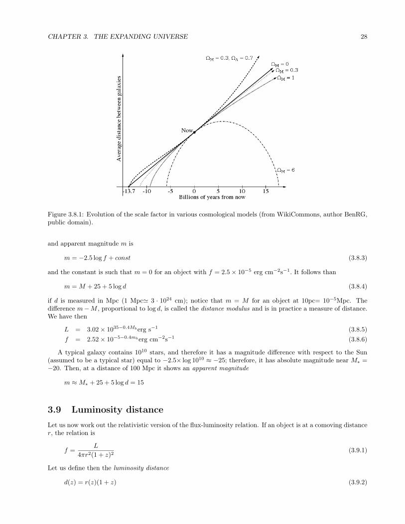
Figure 3.8.1: Evolution of the scale factor in various cosmological models (from WikiCommons, author BenRG,public domain).
and apparent magnitude m is
m = −2.5 log f + const (3.8.3)
and the constant is such that m = 0 for an object with f = 2.5× 10⁻⁵ erg cm−2s−1. It follows than
m = M + 25 + 5 log d (3.8.4)
if d is measured in Mpc (1 Mpc' 3 · 1024 cm); notice that m = M for an object at 10pc= 10−5Mpc. Thedifference m−M , proportional to log d, is called the distance modulus and is in practice a measure of distance.We have then
L = 3.02× 1035−0.4Mberg s−1 (3.8.5)f = 2.52× 10⁻⁵−0.4mberg cm−2s−1 (3.8.6)
A typical galaxy contains 1010 stars, and therefore it has a magnitude difference with respect to the Sun(assumed to be a typical star) equal to −2.5× log 1010 ≈ −25; therefore, it has absolute magnitude near M∗ =−20. Then, at a distance of 100 Mpc it shows an apparent magnitude
m ≈M∗ + 25 + 5 log d = 15
3.9 Luminosity distanceLet us now work out the relativistic version of the flux-luminosity relation. If an object is at a comoving distancer, the relation is
f =L
4πr2(1 + z)2(3.9.1)
Let us define then the luminosity distance
d(z) = r(z)(1 + z) (3.9.2)

CHAPTER 3. THE EXPANDING UNIVERSE 29
so that the Euclidean relation (3.8.2) is formally unchanged. This is by definition the distance that occurs inthe distance modulus relation (m−M) in eq. (3.8.4). The two extra factors (1 + z) in (3.9.1) arise because theemitted energy is redshifted away and because the time interval during which is received, dt0,is a0/a1 times theemission interval dt1. The coordinate distance r(z) is the distance along the null geodesic
ds2 = c2dt2 − a2dr2 = 0 (3.9.3)
In a flat universe (k = 0) we have∫ r
0
dr′ =
∫ t0
t1
cdt
a(t)(3.9.4)
That is
r =
∫ r
0
dr′ = c
∫ t0
t1
dt
a(t)= c
∫ a0
a1
dt
da
da
a= c
∫da
aa= c
∫ a0
a1
da
Ha2(3.9.5)
Using the redshift z we obtain
dz = −da/a2 (3.9.6)
so that
r = c
∫ z
0
dz′
H(z′)(3.9.7)
For a non-flat space we have instead∫ r
0
dr′√1− kr2
=
∫ z
0
dz′
H(z′)(3.9.8)
or, putting H = H0E(z), y = rH0 and Ωk = −k/H20∫ r
0
dy√1 + Ωky2
=
∫ z
0
dz′
E(z′)(3.9.9)
This can be integrated to give
r =1
H0
√|Ωk|
S[√|Ωk|
∫ z
0
dz′
E(z′)] (3.9.10)
where
S(x) =
sin(x) if k = +1
x if k = 0
sinh(x) if k = −1
(3.9.11)
This is quite a general formula. Given any cosmological model (i.e., fixing the parameters Ωr,Ωm,ΩΛ etc) wecan obtain r(z), then d(z) and finally predict the magnitude m(z) that a source of given absolute magnitudeM should have. For instance, in a flat universe with pure matter
H2 = H20a−3 = H2
0 (1 + z)3 (3.9.12)
from which
r(z) = cH−10
∫ z
0
dz(1 + z)−3/2 =2c
H0
[1− (1 + z)−1/2
](3.9.13)
and the luminosity distance is
d(z) =2c
H0
[(1 + z)− (1 + z)1/2
](3.9.14)
CHAPTER 3. THE EXPANDING UNIVERSE 30
Suppose now we have a supernova at z = 1. If its magnitude is M we have that
m(z = 1) = M + 25 + 5 log d(z = 1) = M + 25 + 5 log 3514 = M + 42.7
For a supernova type Ia we have M ≈ −19.5, so that for a flat universe we predict m ≈ 23.2. If we evaluatem(z) for a model with Ωm = 0.3 and ΩΛ = 0.7 we obtain instead m = 23.8. The difference ∆m = 0.6 isdistinguishable with the present data and the best model contains in fact a fraction of cosmological constantaround 70% of the critical one.
We observe finally that r(∞) = 2c/H0 (the big bang distance) and that
c
H0=
300, 000 km/sec100h km/sec/Mpc
= 3, 000Mpc/h
so that r(∞) = 6000 Mpch−1.
Chapter 4
Thermal processes
Quick summary• As the temperature goes down in the past we expect that the various species of particles in the universe
gradually break out of thermal equilibrium.
• In other words, the mean free path from a given interaction between the particles becomes larger thehorizon scale H−1 .
• This phenomenon leads to the annihilation of electrons from radiation at z ≈ 1010 (T ≈ 1MeV), theformation of light atomic nuclei at z ≈ 108 (T ≈ 0.1MeV) and the decoupling of baryons from photons,z ≈ 103 (T ≈ 1eV).
4.1 PreliminariesAlong the universe cosmic history we can identify a number of phases, the first four still hypothetical while thelatter two rather well established:
• Quantum gravity. T ∼ 1019GeV (Planck energy), t ∼ 10−43sec.
• Baryogenesis. 1017GeV < T < 102GeV [perhaps 1015 GeV, t ∼ 10−35sec].
• Electroweak transition. T ∼ 103GeV (mass of weak bosons, Z0,W±).
• Quark-Hadron transition. T ∼ 1GeV (nucleon mass).
• Nucleosynthesis. T ∼ 1MeV , t ∼ 3min (nuclear levels).
• Recombination. T ∼ 10eV , t ∼ 106yr (atomic levels).
The energy scales here indicated are very approximated, sometimes even by an order of magnitude largerthat the real values, due to the very high number of photons per particle (so that a sufficient number of hotphotons still remain even at low temperatures), as we will see in due course. All these phases occur becausethe temperature dropped enough to break reversibility, i.e. to allow some process while forbidding others.For instance, electrons remain in thermodynamic equilibrium with radiation as long as the electron-positronannihilation is compensated by photon pair production, i.e. e−+e+ ↔ γ+γ. But when the average energy of thephotons decreases below the 0.5 MeV needed for the electron mass, the pair production becomes forbidden andthe residual pair annihilation raises the photon temperature. More in general, denoting with Γ the interactionrate (probability of events per unit time), we say that there is a freezing for that particular interaction whenΓ H or, in other words, when the interaction rate is smaller than the expansion rate, or again, equivalently,when the mean free path for the interaction is much larger than the cosmic horizon cH−1. We discuss now insome detail three thermal events: neutrino abundance, primordial nucleosynthesis, and recombination.
31

CHAPTER 4. THERMAL PROCESSES 32
In the following we need some integrals of the thermal equilibrium distribution of a particle A with gAinternal degrees of freedom as a function of energy E =
√k2 +m2, momentum k, mass m and temperature T
(we assume ~ = c = kB = 1), given by
f(k, t)d3k =gA
(2π)3[eE−µAT (t) ± 1]−1d3k
where µA is the chemical potential of that species (defined as the change in total energy when varying thenumber of particles keeping constant entropy, volume and number of other particles). The distribution f isnormalized in such a way that the integral over all momenta is the number density. It’s important to note thatin every reaction, the total chemical potential is preserved. The sign ± refers to bosons (−, Bose-Einstein) orfermions (+, Fermi-Dirac). From this we derive the number density distribution n, the energy density ρ, thepressure p as a function of T :
n =
∫f(k)d3k =
g
2π2
∫(E2 −m2)1/2EdE
eE−µAT ± 1
ρ =
∫Ef(k)d3k =
g
2π2
∫(E2 −m2)1/2E2dE
eE−µAT ± 1
p =
∫k2
3Ef(k)d3k =
g
6π2
∫(E2 −m2)3/2dE
eE−µAT ± 1
(4.1.1)
(notice that d3k integrated over the angles gives 4πk2dk = 4π(E2 −m2)1/2EdE).The third equation has been obtained as follows. In Special Relativity, one has the general relations p =
〈vk〉/3 and v = k/E. The average 〈〉 is meant as an average over a unit-normalized distribution, i.e. V f(k)/N ,so for a mono-particle ideal gas with p = 2EK/3V = Nmv2/(3V ) = Nvk/(3V ) = Nk2/(3EV ) we have indeed
〈p〉 = 〈Nk2
3EV〉 =
∫k2
3Ef(k)d3k (4.1.2)
Applying the first equation to the photons, for which g = 2 and m = µ = 0, we obtain the numerical density
nγ =2ζ(3)
π2T 3 (4.1.3)
(where the Riemann function ζ is defined as ζ(x) = Γ(x)−1∫∞
0ux−1
eu−1du and ζ(3) ≈ 1.2). The same result, with afactor 3/4, is valid for a relativistic fermionic component, e.g. neutrinos. To recover standard units, one shouldmultiply by (kB/~c)3. The energy density is
ργ = gγπ2
30T 4 (4.1.4)
where gγ = 2 for the photons (and a factor k4B/(~c)3 to recover standard units). Eq. (4.1.4) holds also for every
relativistic components (T m), with the factor 7/8 for fermions. From the pressure relation, we find p = ρ/3in the relativistic regime.
4.2 The abundance of cosmic neutrinos(In this section I followed the approach in Piattella, Lecture Notes in Cosmology, Springer.) Since the Universeis a closed system, the total entropy S is constant. The specific entropy s = S/V decreases therefore as a−3,so that sa3 is constant. Let us now find an expression for the specific entropy. We begin with the first law ofthermodynamics
TdS = pdV + dU (4.2.1)
Putting U = ρV and constant entropy, dS = 0, this becomes
TdS = (ρ+ p)dV + V dρ = 0 (4.2.2)
CHAPTER 4. THERMAL PROCESSES 33
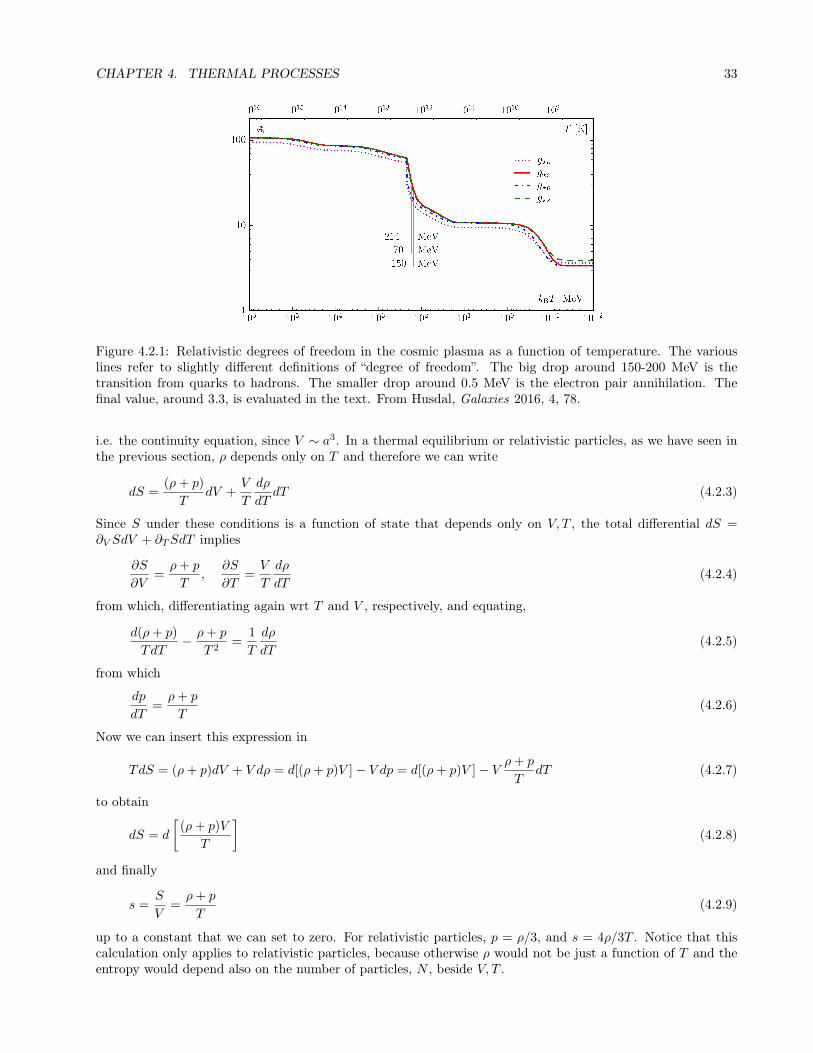
Figure 4.2.1: Relativistic degrees of freedom in the cosmic plasma as a function of temperature. The variouslines refer to slightly different definitions of “degree of freedom”. The big drop around 150-200 MeV is thetransition from quarks to hadrons. The smaller drop around 0.5 MeV is the electron pair annihilation. Thefinal value, around 3.3, is evaluated in the text. From Husdal, Galaxies 2016, 4, 78.
i.e. the continuity equation, since V ∼ a3. In a thermal equilibrium or relativistic particles, as we have seen inthe previous section, ρ depends only on T and therefore we can write
dS =(ρ+ p)
TdV +
V
T
dρ
dTdT (4.2.3)
Since S under these conditions is a function of state that depends only on V, T , the total differential dS =∂V SdV + ∂TSdT implies
∂S
∂V=ρ+ p
T,
∂S
∂T=V
T
dρ
dT(4.2.4)
from which, differentiating again wrt T and V , respectively, and equating,
d(ρ+ p)
TdT− ρ+ p
T 2=
1
T
dρ
dT(4.2.5)
from which
dp
dT=ρ+ p
T(4.2.6)
Now we can insert this expression in
TdS = (ρ+ p)dV + V dρ = d[(ρ+ p)V ]− V dp = d[(ρ+ p)V ]− V ρ+ p
TdT (4.2.7)
to obtain
dS = d
[(ρ+ p)V
T
](4.2.8)
and finally
s =S
V=ρ+ p
T(4.2.9)
up to a constant that we can set to zero. For relativistic particles, p = ρ/3, and s = 4ρ/3T . Notice that thiscalculation only applies to relativistic particles, because otherwise ρ would not be just a function of T and theentropy would depend also on the number of particles, N , beside V, T .

CHAPTER 4. THERMAL PROCESSES 34
Neutrinos and photons do not interact, so if they start with the same temperature at very early times whenT 1MeV (as expected because the equilibrium is realized through weak interactions), they should maintain itforever. However, photons are heated by electron pair production, so we expect a temperature mismatch below0.5 MeV, right before nucleosynthesis. To determine this, we can evaluate s for relativistic bosons (photons)and fermions (neutrinos and electrons). From (4.1.4) we have
sν =4ρ
3T=
7
8gν
4π2
3 · 30T 3 =
7
8gν
2π2
45T 3 (4.2.10)
sγ = gγ2π2
45T 3 (4.2.11)
where the degrees of freedom are gγ = 2 for photons (and also for electrons and positrons), and 2gνNν for Nνspecies of neutrinos (i.e. Nν times gν for neutrinos and gν for antineutrinos). In the standard particle physicsmodel, each neutrino type has only one dof instead of two, since right-handed neutrinos, if they exist at all,interact only with gravity. At T 0.5 MeV, i.e. before pair annihilation, all species have the same temperature,so one has for the relativistic dofs (photons plus electrons/positrons plus neutrinos/antineutrinos)
sb =2π2
45T 3b (2 +
7
8· 4 +
7
8· 2Nνgν) (4.2.12)
After pair production stops, the temperatures of the surviving species, photons and neutrinos, will be different,so we have instead
sa =2π2
45(2T 3
γ +7
8· 2gνNνT 3
ν ) (4.2.13)
Since sa3 is constant, we have
(abTb)3[2 +
7
8· 4 +
7
8· 2gνNν ] = (aaTν)3[2
(TγTν
)3
+7
8· 2gνNν ] (4.2.14)
Now the neutrino temperature goes always as 1/a since they are not heated by electron pair annihilation, soabTb = aaTν and finally
TνTγ
=
(4
11
)1/3
≈ 0.714 (4.2.15)
This ratio is maintained forever after. Since today Tγ ≈ 2.7K, the unobservable Tν should be around 1.9 K.As a consequence, since ργ , ρν ∼ T 4, we have
ρνtot = ρν+ν =7
8Nνgν
(4
11
)4/3
ργ (4.2.16)
A recent estimation of Nνgν via CMB gives roughly Nνgν ≈ 3 ± 0.3, consistent with the three families in thestandard particle physics model and gν = 1, so that ρνtot ≈ 0.68ργ . The total relativistic energy density today istherefore ρνtot + ργ ≈ 1.68ργ ; in practice, one can simply say that instead of gγ = 2, today’s relativistic degreesof freedom are g∗γ = 2 · 1.68 = 3.36.
Similarly, since there are 2Nν species of neutrinos plus antineutrinos (from now on, ν refers to the sum ofν, ν), and writing nγ(T ) = AT 3, their number density is
nν =3
4(2Nν)nγ(Tν) =
3
2NνAT
3ν =
3
2NνAT
3γ
(TνTγ
)1/3
=3
2Nν
(4
11
)AT 3
γ =6
11Nνnγ(Tγ) (4.2.17)
This gives roughly 340 neutrinos per cm3. If the neutrinos have a small mass mν < 1eV, as it appears fromthe current constraints from solar neutrino oscillations and cosmological observations, they have become non-relativistic just recently, so the description above remains substantially intact. However, their energy densitynow would be nνmν where the average mass is mν =
∑mν/Nν . This gives
ρν,0 =6
11nγ∑
mν (4.2.18)

CHAPTER 4. THERMAL PROCESSES 35
and their cosmic fraction
Ων,0 =8πG
3H20
6
11nγ∑
mν ≈∑mν
93h2eV(4.2.19)
(here h is the dimensionless Hubble constant). With h ≈ 0.7, three neutrinos of 5 eV each would compose allof the observed dark matter. Unfortunately, this simple explanation for the dark matter is today ruled out onseveral grounds. Massive neutrinos (at least in the standard scenario) can compose less than one percent of thetotal energy content. More details on possible candidates of dark matter will be discussed later on.
4.3 Primordial nucleosynthesisThe binding energy of nuclei is at the MeV scale. Therefore, at temperatures much higher than 1 MeV, protonsand neutrons cannot combine to form heavier nuclei like deuterium, helium etc. because the hot thermal bathwould immediately reionize them. Since protons are slightly lighter than neutrons, in an equilibrium Boltzmanndistribution with temperature T ≈ mn−mp ≈ 1.3MeV ≈ 1.5 ·1010 K there will be more protons than neutrons.
Already at TD ≈ 0.7 MeV neutrons and protons are no longer in equilibrium under reactions like n+ νe ↔p+ e− and their numerical ratio n/p freezes at
nnnp
= e−∆mTD ≈ 1
6(4.3.1)
Today’s temperature 3K corresponds to 2.4 · 10−4eV, so at 0.7 MeV the scale factor was aD = T3K/T0.7MeV ≈3.4 · 10−10. Since we are deep into the radiation era H = H0
√Ωγa
−2, so this corresponds to a time after bigbang
tD =1
H0
√Ωγ
∫ ∞zD
dz
(1 + z)3=
1
2H0
√Ωγ(1 + zD)2
≈ 10s (4.3.2)
In the mean time, a fraction of neutrons decayed spontaneously (lifetime 900 sec) so that one can estimaten/p = 1/7 at around 0.1 MeV, when most of the nucleosynthesis process can be considered completed, as willsee in the next section. If in a first approximation we assume that all the neutrons nn end up into in nn/2nuclei of 4He (which is a very stable nucleus), we can estimate the mass fraction in Helium as
Y =4(nn/2)
nn + np≈ 0.25
a value which is very close to the observed one.In reality, one should consider a network of reactions, the most important of which are (Fig. 4.3.1) (D =2H=
deuterium, T =3H= tritium)
p+ n → D + γ
D + p → 3He+ γ
D +D → 3He+ n
D +D → T + p3He+ n → T + p
3He+D → 4He+ p
T +D → 4He+ n
All the other higher mass nuclei have much lower abundances, especially after atomic mass 5 and 8, for whichthe nuclei are unstable. Reactions like 4He + T →7 Li+ γ or 3He +4 He →7 Be + γ do occur but with muchreduced probability. So hydrogen, helium, lithium and beryllium are essentially the only elements primordiallyproduced.
The nuclei abundance depends critically on the baryon/photon ratio η ≈ 10−8Ωbh2 (see next section) because
if there are more photons then the time at which nuclei can form will be delayed due to the high energy tail of

CHAPTER 4. THERMAL PROCESSES 36
Figure 4.3.1: Big bang nucleosynthesis main reactions (from WikiCommons, author Pamputt).
the photon distribution (see Eq (4.4.12) below). The quantity η is constant since both the number of baryonsand photons scale as a−3. The number of photons today can be directly measured from the CMB black bodytemperature T = 2.7K. Therefore from η we can obtain the density of baryons in the universe, i.e. Ωbh
2.Comparing with the theoretical predictions with the observed element abundances in the oldest stars (Fig.4.3.2) we obtain
Ωbh2 = 0.022± 0.002
In combination with the estimates of h ≈ 0.7 one obtains Ωb ≈ 0.05. This shows that the cosmological baryondensity is much smaller than the critical one.
4.4 Primordial nucleosynthesis, more detailsSince the baryonic density decreases as T 3 and it is now (we put mB ≈ 1GeV )
nB =ρBmBc2
= Ωbρc
mBc2= (Ωbh
2)10−47GeV 3 (4.4.1)
there is a constant ratio baryons/photons equal to
η =nBnγ
= 2.68 · 10−8(Ωbh2) (4.4.2)
(where Ωb is the present value). We need also the low temperature limit T m of eqs. (4.1.1)
n = g(mT
2π)3/2e−
m−µT (4.4.3)
ρ = nm (4.4.4)p = nT ρ (4.4.5)
(one has to expand√m2 + k2 ≈ m(1+k2/2m2) in the exponential). Consider now the universe at a temperature
T ∼ 1 MeV. Since the binding energy of light nuclei as 2H,3H,3He is 2.22, 6.92, 7.72 MeV, respectively, atT ∼ 1 Mev the nuclei should be able to form, out of the neutron-proton plasma: as we show now, however, the
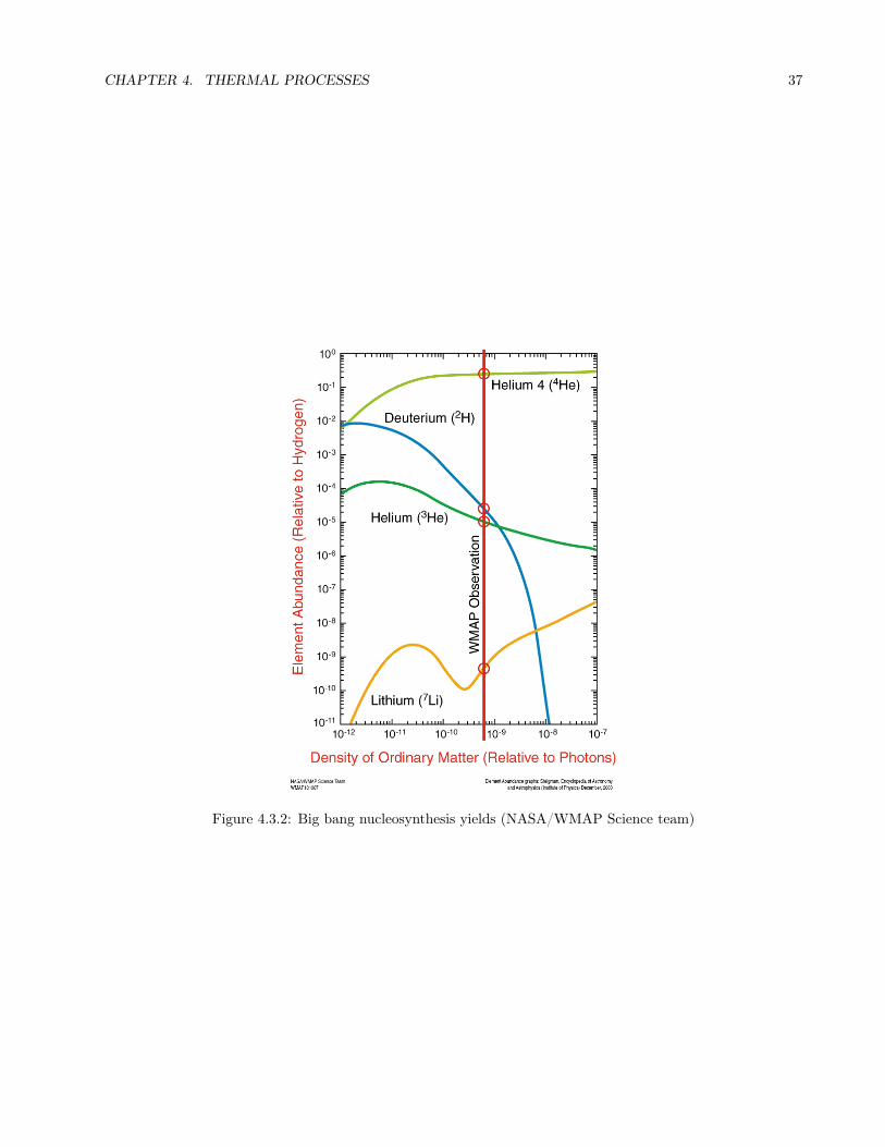
CHAPTER 4. THERMAL PROCESSES 37
Figure 4.3.2: Big bang nucleosynthesis yields (NASA/WMAP Science team)

CHAPTER 4. THERMAL PROCESSES 38
actual temperature of formation is quite lower, due to the high photon-to-baryon ratio. In a thermal equilibriumtheir distributions are (g = 2)
nn = 2(mBT
2π)3/2e−
mn−µnT (4.4.6)
np = 2(mBT
2π)3/2e−
mp−µpT (4.4.7)
where mB ≈ mn ≈ mp. Let us consider now a reaction in which a nucleus ANZ with Z protons and A − Zneutrons forms. The distribution of such a nucleus in thermal equilibrium is, similarly, (we use the subscript Afor the nucleus)
nA = gA(mAT
2π)3/2e−
mA−µAT (4.4.8)
For the preservation of chemical potentials (i.e. conservation of energy) we have
µA = Zµp + (A− Z)µn (4.4.9)
This allows us to write the number density nA of the nuclei as a function of mn,p, nn,p:
nA = gA2−AA3/2(mBT
2π)3(1−A)/2nZp n
A−Zn e
BAT (4.4.10)
BA ≡ Zmp + (A− Z)mn −mA (4.4.11)
where BA is the (positive) binding energy of the nucleus, which as already mentioned is of order 1 MeV or larger.Let us define the mass fraction of nucleus N with respect to the baryonic density nB = ηnγ = η2ζ(3)T 3/π2 :
XA =AnAnB
and similarly Xn,p = nn,p/nB . Then we obtain finally,
XA = F (A)(T
mB)3(A−1)/2ηA−1XZ
p XA−Zn eBA/T (4.4.12)
where
F (A) = gAA5/2ζ(3)A−1π(1−A)/22(3A−5)/2 (4.4.13)
is a factor of order unity. From (4.4.12) we see that the production of the nucleus A, defined as the epoch atwhich the value of XA ∼ 1 is reached, can only occur at temperatures TA much lower than BA, because of thesmall factor ηA−1, i.e. because of the large number of photons per baryon present (high entropy). In otherwords, one needs to assume a very small η in order to obtain small temperatures TA, which in turn agree withthe observed nuclei abundance. Neglecting all factors of order unity, and also putting Xn,p ≈ 1, we can writenumerically
TA ≈BA/(A− 1)
log η−1 + 1.5 log(mB/T )(4.4.14)
We obtain then TA ≈ 0.07, 0.11, 0.28MeV for 2H,3He,4He, i.e. values much lower than their respective bindingenergies. Temperatures of the order of 0.1 MeV imply a = T0/TA ≈ 10−8 and therefore znucl ≈ 108 . You canalso show that tnucl ≈ 102sec.

CHAPTER 4. THERMAL PROCESSES 39
4.5 Matter-radiation decouplingLet us apply now similar arguments at a lower temperature, T ≈ 10 eV, at which we expect that hydrogenatoms, whose binding energy is 13.6 eV, can form. At higher temperatures, the Compton and bremsstrahlunginteractions keep the thermal equilibrium between matter and radiation. In this case, just as before, we haveT m and we can write
ni = 2(miT
2π)3/2e−
mi−µiT
where i =electrons, protons and hydrogen atoms. In the reaction p + e → nH + γ the chemical equilibriumrequires µp + µe = µH and therefore, as in the previous case, we obtain
nH =gHgpge
npne
(meT
2π
)−3/2
eB/T
where gp,e = 2 and gH = 4, and B = mp + me − mH = 13.6 eV. We define now the ionization fraction foreach species, xi = ni/nB . Since np = ne, and np + nH = nB we have xp = xe and xH = (nH/nB) = 1 − xe.Therefore we obtain a relation for xe (Saha equation):
1− xex2e
=4√
2ζ(3)√π
η
(T
me
)3/2
eB/T ≈ 3.84η
(T
me
)3/2
eB/T
From this equation we can track the evolution of the ionization fraction xe(T ). The lower is xe, the moreadvanced the recombination process is. For instance, we’ll have an almost total recombination xe = 0.1 at thetemperature τ ≡ T/1eV where (by iteration)
τ−1 = 3.084− 0.00735 log(Ωbh2)
therefore since z = (T/T2.7K) = τ(1eV/T2.7K) ≈ 4200τ we have the recombination redshift
z ≈ 1367(1− 0.024 log Ωbh2)−1
Then we see that the recombination of electrons and protons into hydrogen atoms can be said to be completed atT ≈ 0.3eV, i.e. at a temperature quite smaller then the typical binding energy, analogously to the nucleosynthesiscase.
When neutral atoms form, radiation cannot keep thermal equilibrium with matter. At some temperatureTdec the Thomson interaction becomes smaller than the expansion rate H (or in other words the photon meanfree path becomes of the order of the Hubble radius) and matter decouples. This happens roughly at
zdec ≈ 1100
This is therefore the instant at which the photons last scatter off the electrons and protons and begin theirfree travel through space, some of them ultimately to be captured as CMB photons by our detectors.
Chapter 5
The distance ladder
Quick summary• Distances are measured with a variety of ways, valid for different ranges and for different type of sources.
• The basic method, on which practically all the others rely, is the parallax method, valid up to 50 kpc, i.e.the distance of nearby satellite galaxies.
• One of the most important method to extend the distance range is based on the period-luminosity-colorrelation of the Cepheid variable stars, extending to 20 or so Mpc.
• Beside this distance one has to rely either on the Tully-Fisher and Fundamental Plane relation for spiraland elliptical galaxies, respectively, or on the standardized supernovae Ia, or on a number of alternativebut less precise techniques.
• Using a combination of all these methods, the Hubble constant has been recently measured to be H0 ≈72± 3 km/sec/Mpc.
5.1 The parallax methodThe basic method to determine distance is the parallax method. All the other methods build on this first step.The idea (first successfully used in 1838 by Friedrich Bessel) is to find the change in direction to a nearby star,with respect to the Sun (or, better, to very distant stars), when the Earth is at opposite locations on the ecliptic(i.e. 2A.U.= 300 million kilometers apart). If there is no change, the star is at infinity. Simple trigonometryshows that if the parallax is 1 arcsec, then the star is roughly 2 ·1013km away, i.e. (by definition) 1 parsec= 3.26light years. The distance in general is then
d =1pc
θ[arcsec](5.1.1)
The satellites Hipparcos (1989) and Gaia (2013) measured parallaxes down to 10µarcsec=10−5arcsec, reachingtherefore distances of the order of 100 kpc, much beyond the limits of the Milky Way (which has a size of 10kpcroughly). In particular the distance to the Large Magellanic Cloud (LMC) has been found to be
DLMC ≈ (50± 1)kpc (5.1.2)
This is a very important value since all the other methods give only relative measurements (i.e. are calibratedultimately through the parallax method).
5.2 CepheidsThe second most important method is based on the variable stars known as Cepheids (from the constellationwhere the first example has been observed). These variable stars are red giant near the end of their life. The He
40

CHAPTER 5. THE DISTANCE LADDER 41
Figure 5.2.1: Period-Luminosity relation for Magellanic Cloud Cepheid variable stars; data from Storm et al.2011, A&A, 534. (Wikicommons, author: Dbenford)
envelope is ionized when the temperature is high; a ionized He is highly opaque to radiation coming from the corewhich therefore is trapped and expand the envelope, making the star brighter. When the envelope expands,the temperature drops and the helium recombines (de-ionizes) so the envelope becomes more transparent.The radiation flows out, the pressure decreases, the envelope contracts, and the star becomes dimmer. Thecontraction however increases the temperature again and the cycle restarts, lasting from days to several weeks.The series of oscillations is very stable for some thousand years. Henrietta Leavitt around 1910 found that theperiod is larger is the peak absolute luminosity is larger according to roughly
L ∼ P 1.3 (5.2.1)
In order to fix the proportionality constant in this relation (and to ensure that is really universal, i.e. it appliesto all Cepheids), one needs to calibrate it, i.e. to measure the luminosity and the period for a number of nearbyCepheids for which we know the distance (and therefore the absolute magnitude) with the parallax method.This crucial step is necessary for all the methods we are going to discuss.
A recent determination from the Hubble Space Telescope on nearby Cepheids found (P is in days)
MV = (−3.43± 0.11)(log10(P )− 1)− (5.93± 0.03) (5.2.2)
This can used to determine distances directly as
5 log d[Mpc] + 25 = V + 3.746(log10(P )− 1)− 2.523(V − I) + 5.959 (5.2.3)
where V, I are the apparent magnitudes in two different wavebands, and a color correction due to the influenceof metallicity on the period-luminosity relation, proportional to V − I, is included (Fig. 5.2.1)
Recently, Cepheids have been identified in galaxies of the Virgo cluster (15 Mpc away) and, still in progress, inthe Coma cluster (65 Mpc/h). The Cepheids in the Virgo cluster have been fundamental in reducing drasticallythe error in the measurement of H0 (Fig. 5.2.2)
5.3 Planetary nebulaePlanetary nebulae (PN) are stars with an extended envelope of hot gas ionized by the star itself. They appearedto early astronomers as “planets” because of their disk-like extended form. They are relatively easy to identifybecause most of the emission is in some specific line, eg. OIII. Their luminosity function (i.e. the functionΦPN that gives how many PN one has in a luminosity range dL, dNPN = ΦPNdL) has a sharp cut-off at highluminosity (see Fig. 5.3.1). Essentially, no PN is found with absolute magnitude brighter than -5. If one cancollect many PN in a galaxy so as to determine this cutoff with good precision, then the value of the brightestPN can be used as a distance indicator.

CHAPTER 5. THE DISTANCE LADDER 42
Figure 5.2.2: Hubble constant from the Cepheid method (Freedman et al., Ap. J., Volume 553, Issue 1, pp.47-72, 2001. © AAS. Reproduced with permission).
Figure 5.3.1: Luminosity functions of planetary nebulae in a sample of galaxies. Notice the sharp cut-off at highluminosity. (From Ciardullo et al. 2002, astro-ph/0206177, Astrophys.J. 577 (2002) 31-50. © AAS. Reproducedwith permission.)

CHAPTER 5. THE DISTANCE LADDER 43
5.4 Surface Brightness FluctuationsAnother method exploits the fact that in a random process the fluctuations have a variance proportional to thenumber of trials. For instance, if we throw randomly balls inside a grid, without aiming at any cell in particular,and if N is the average number of balls per cell, the typical fluctuation (i.e. the square root of the variance) ofthe number of balls is
√N . More exactly, the variance
σ2 =1
nc
nc∑i
(Ni − N)2 ≈ N (5.4.1)
where nc is the number of cells in the grid and Ni the count in the i-th cell. The relation is exact in the limitof an infinite number of cells.
So in a galaxy one can divide the image into many little pixels and estimate the fluctuations in the surfacebrightness (SFB) (i.e. the flux divided by area of the pixel). The variance σ2
SBF in SBF goes like the averagenumber of stars in the pixel N , and the fluctuation as
√N . The total luminosity of the galaxy however goes
obviously like N . So we have
L = ασ2SBF (5.4.2)
and we expect α to be a universal quantity since the random events that distributed stars in a galaxy shouldnot depend on the galaxy distance.
Once again, if one estimates α with a sample of known distance and therefore known luminosity, one can usethis relation for distant galaxies. Of course the calibration will be tighter if one uses galaxies of the same type
5.5 Tully-Fisher relation and the Fundamental PlaneSpiral galaxy stars have little random motion and large (≈ 200 − 300 km/sec) rotational velocity; in contrast,elliptical galaxy stars have little rotational velocities (less then 100 km/sec) but large random motion (severalhundreds of km/sec). In both cases, the velocities seem correlated with the absolute luminosity: brightergalaxies (therefore very likely more massive) contain faster stars. This is entirely to be expected because of thevirial theorem that links (twice) the average kinetic energy to the average gravitational potential energy
〈v2〉 = 〈Φ〉 =GM
Rvir(5.5.1)
The velocity of stars with respect to the galaxy center is estimated by measuring the width of emission lines: aline emitted by several sources with some velocity dispersion will be a superposition of several lines with slightlydisplaced wavelength due to Doppler effect: the result is a wider line (for ellipticals) or a double-peaked line(for spirals, where stars are either moving relatively towards us or away from us), see Fig. 5.5.1.
The Tully-Fisher relation valid for spiral galaxies read
L ∼ σαrot (5.5.2)
with α ≈ 3.5− 4, depending on the band at which L is measured (Fig. 5.5.2).For elliptical galaxies one finds empirically a number of relations among four quantities: the effective radius
Re, the surface brightness within that radius Ie, the luminosity L and the velocity dispersion σV . In particularone has the Faber-Jackson relation
L ∼ σαV (5.5.3)α ≈ 3− 4 (5.5.4)
and also
Re ∼ I−0.83±0.08e (5.5.5)
Moreover, by definition, Le = πR2eIe. One finds also Ie ∼ L−3/2 (brighter ellipticals have smaller surface
brightness) and the fundamental plane for ellipticals, i.e. a relation among three of the four variables, forinstance
R = c · σaV Ib (5.5.6)

CHAPTER 5. THE DISTANCE LADDER 44
Figure 5.5.1: Double-peaked line from a spiral galaxy. (From the websitehttps://www.ipnl.in2p3.fr/projet/cosmicflows/).
Figure 5.5.2: Tully-Fisher relation in the IR band around 3.6µm (Sorce et al., 2013ApJ...765...94S, © AAS.Reproduced with permission) for galaxies up to roughly 200 Mpc.
where σV is in km/sec and R is in kpc, a, b, c are constants, or equivalently (redefining b, c)
logRe = a log σV + bµ+ c (5.5.7)
where µ = −2.5 log I (measured in mag arcsec−2, analogously to the definition of magnitudes). A recentcalibration through 1430 nearby galaxies gives a ≈ 1.5, b ≈ 0.3 c ≈ −9 (La Barbera et al. ApJ 2008).
Once again, from the absolute luminosity and the measured flux, or from the absolute radius and themeasured angular size, one can obtain the luminosity or the angular diameter distance, respectively.
5.6 Supernovae IaIn 1998 Riess et al. [High-redshift Supernova Search Team (HSST)] and Perlmutter et al. [Supernova CosmologyProject (SCP)] independently reported the late-time cosmic acceleration by observing distant supernovae of typeIa (SN Ia). Up to 1998 Riess et al. had discovered 16 high-redshift SN Ia together with 34 nearby supernovae,while Perlmutter et al. had found 42 supernovae in the redshift range z = 0.18-0.83.
CHAPTER 5. THE DISTANCE LADDER 45
The explosion of supernovae is extremely luminous and causes a burst of radiation. The supernovae can beclassified according to the absorption lines of chemical elements (Fig. 5.6.1). If the spectrum of a supernovaincludes a spectral line of hydrogen, it is classified Type II. Otherwise it is called Type I. If a supernova containsan absorption line of singly-ionized silicon, it is further classified Type Ia (note that Type Ib contains a line ofhelium, whereas Type Ic lacks the lines of both silicon and helium). The explosion of Type Ia occurs when themass of a white dwarf in a binary system exceeds the Chandrasekhar limit by absorbing gas from a companionstar (Fig. 5.6.2). A white dwarf is a relatively simple object which undergoes passive cooling in equilibriumbetween gravity and the electron degeneracy pressure, without nuclear fusion. When the mass exceeds thelimit, the star collapses but contrary to normal stars the degeneracy pressure cannot increase because it isindependent of temperature. The temperature increases so fast that the heavy nuclei (mostly C,O) fuse (thatis why these supernovae are also called thermonuclear SNa) and the thermal motion of the particles exceedsthe escape speed and the star explodes. Ultimately the typical form of the SN Ia lightcurve depends on thesubsequent radioactive decay of the Ni, Fe elements from the exploding envelope, which takes almost a monthbefore fading off. The Chandrasekhar limit depends only on fundamental constants
MCh = c ·(~cG
)3/21
(µemH)2≈ M3
P
m2p
≈ 1.4M (5.6.1)
where MP is the Planck mass, c is a constant of order unity, mp is the proton mass, µe is the average molecularweight per electron (it depends then on the chemical composition of the star). One expects therefore that theenergy emitted by the disruption of such an object is an almost universal constant. To test this hypothesis isnecessary as usual a calibration, i.e. a sample of nearby SNIa of which we know the distance with other means,and from which we can obtain therefore their absolute magnitude MSN . Then the SN Ia become a kind of“standard candle” by which luminosity distance can be measured observationally.
In reality things are more complicated than this simple view. The intrinsic spread in absolute magnitudesis actually too large to produce stringent cosmological constraints. However, at the end of the 1990s, a highquality sample of “local” (i.e. z 1) supernovae allowed to correlate the absolute magnitude with the width ofthe light curve: brighter supernovae have a broader light curve, roughly L ∼ τ1.7 if τ is a measure of the widthof the lightcurve (Fig. 5.6.3). By measuring at the same time the apparent magnitude and the light curve it ispossible therefore to predict the absolute magnitude. Although in the following we refer to a universal SN Iaabsolute magnitude, we always mean the magnitude corrected for the light curve width.
Since the (corrected) peak absolute magnitude MSN is the same for any SN Ia under the assumption ofstandard candles, the luminosity distance dL(z) is obtained from measuring m and the relation
5 log dL = m−MSN − 25 (5.6.2)
At small redshifts, dL = cz/H0 and we can therefore infer H0. At large redshifts SNIa can be employed tomeasure dL(z) as a function of cosmological parameters, as we will see in another chapter.

CHAPTER 5. THE DISTANCE LADDER 46
Figure 5.6.1: Classification of SN types. The different spectra make possible a reliable identification of SN Ia(from supernova.lbl.gov).
Figure 5.6.2: Pictorial representation of a white dwarf accreting matter from a red giant companion and thenexploding as a SNIa (Image: NASA/CXC/M Weiss).

CHAPTER 5. THE DISTANCE LADDER 47
Figure 5.6.3: Calibration of nearby SNIa. Above: several slightly different lightcurves: brighter SN have a morestretched lightcurve than dimmer ones. Below: “standardized” lightcurve obtained by a stretch factor appliedto the lightcurves (Hamuy et al. 1996, from supernova.lbl.gov).

Chapter 6
Accelerated expansion
Quick summary• Supernovae Ia are probably the thermonuclear explosion of white dwarfs accreting matter near or beyond
the Chandrasekhar mass from a companion star
• At the luminosity peak, SNIa are as bright as an entire galaxy; the light curve fades away in a monthroughly
• Since the Chandrasekhar mass depends only on fundamental constants, one could reasonably expect thatthe energy emitted during the explosion is roughly constant
• This expectation is confirmed by observations of local SNIa; a correction of the peak luminosity with thelight curve width makes the SNIa excellent standard candles
• Since they can be seen at very large distances, SNIa can be used as distance indicator to z ≈ 1
• In 1998, the Hubble diagram of SNIa showed for the first time an accelerated expansion of the universe,favoring the existence of a large component of a cosmological constant or dark energy; this discovery wasawarded the Nobel Prize in 2011
• There are many models of dark energy that expand upon the idea of a large, weakly clustered, unseen,energy component with negative pressure
6.1 SNIa at high redshiftsa
In 1998 Riess et al. and Perlmutter et al. released observational data of the apparent luminosity of high-redshiftType Ia supernovae (0.2 . z . 0.8). The data of low-redshift regions (z < 0.1) reported previously was alsoused in their analysis. Let us pick up a few examples of data to understand how the luminosity distance isknown observationally. First, consider two data of the apparent magnitudes in the low redshift region of SNIa: (i) 1990O: m = 16.26 (z = 0.03) and (ii) 1992bg: m = 16.66 (z = 0.036). Since the luminosity distancein the region z 1 is well approximated by dL ' cz/H0, the absolute magnitude M is known. We take thevalue h = 0.7 for the Hubble constant. We then obtain M = −19.29 and M = −19.28 for 1990O and 1992bg,respectively. This shows that the absolute luminosity of SN Ia is nearly constant (M ' −19), as we alreadymentioned.
Let us next use the high-redshift data reported by Perlmutter et al. . Consider the two SN Ia data of theapparent magnitudes: (a) 1997R: m = 23.83 (z = 0.657), (b) 1995ck: m = 23.57 (z = 0.656). Employing thevalue M = −19.15 for the absolute magnitude, we find that the luminosity distance is given by H0dL/c = 0.920for 1997R and H0dL/c = 0.817 for 1995ck. Notice that the approximation dL ' cz/H0 is no longer valid in the
aAdapted from Amendola & Tsujikawa, Dark Energy. Theory and Observations, CUP 2010.
48

CHAPTER 6. ACCELERATED EXPANSION 49
0 . 0
1 . 0
2 . 0
3 . 0
4 . 0
5 . 0
6 . 0
7 . 0
8 . 0
0 0 . 5 1 1 . 5 2 2 . 5 3 3 . 5 4
Flat with WDE
= 0
Open with WK
= 0.0085, WDE
= 0
Flat with WDE
= 0.7
H0
dL
/c
z
Figure 6.0.1: The luminosity distance dL versus the redshift z for three cases: (a) a flat universe without darkenergy, (b) an open universe (Ω(0)
K = 0.0085) without dark energy, and (c) a flat universe with the cosmologicalconstant (Ω(0)
DE = 0.7 and wDE = −1). The presence of dark energy leads to a larger luminosity distance relativeto the case without it. In the open universe the luminosity distance also gets larger than that in the flat universe.
Calan/Tololo
(Hamuy et al,
A.J. 1996)
Supernova
Cosmology
Project
eff
ecti
ve m
B
(0.5,0.5) (0, 0)
( 1, 0 ) (1, 0)(1.5,–0.5) (2, 0)
(ΩΜ,ΩΛ) =
( 0, 1 )
Fla
t
Λ =
0
redshift z
14
16
18
20
22
24
26
0.02 0.05 0.1 0.2 0.5 1.00.02 0.05 0.1 0.2 0.5 1.0
Figure 6.1.1: The effective apparent luminosity mB versus the redshift z for 42 high-redshift SN Ia from theSCP and 18 low-redshift SN Ia from the Calan/Tololo Supernova Survey. The solid curves are the theoreticalprediction for mB for a number of cosmological models without the cosmological constant: (Ω
(0)m ,Ω
(0)Λ ) = (0, 0)
(top), (1, 0) (middle), and (2, 0) (bottom). The dashed curves correspond to a number of flat cosmologicalmodels: (Ω
(0)m ,Ω
(0)Λ ) = (0, 1) (top), (0.5, 0.5) (second from top), (1, 0) (third from top), and (1.5,−0.5) (bottom).
From Perlmutter et al. 1998.

CHAPTER 6. ACCELERATED EXPANSION 50
high-redshift regime. Let us consider a flat universe with a dark energy equation of state wDE = −1 (i.e. thecosmological constant). Since E(z) = [Ω
(0)m (1 + z)3 + Ω
(0)DE]1/2 in this case, the luminosity distance reads
dL(z) =c(1 + z)
H0
∫ z
0
dz
[(1− Ω(0)DE)(1 + z)3 + Ω
(0)DE]1/2
, (6.1.1)
which can be evaluated numerically for given Ω(0)DE. In order to satisfy the observational data (H0/c)dL(z =
0.657) = 0.920 for 1997R, we require that Ω(0)DE = 0.70. Similarly we get Ω
(0)DE = 0.38 from the 1995ck data.
Both data indicate the existence of dark energy.Since observational data are prone to statistical and systematic errors, a few data points are not enough to
conclude that the present universe is accelerating. Using 42 high-redshift SN Ia at redshifts between 0.18 and0.83 together with 18 low-redshift SN Ia data from the Calan/Tololo Supernova Survey, Perlmutter et al. (1998)showed that the cosmological constant is present at the 99 % confidence level. They also found that the openuniverse without the cosmological constant does not fit the data well. From Eq. (3.8.4) the apparent luminositym gets larger for increasing luminosity distance dL. Figure 6.1.1 shows that the observational data in the highredshift regime favor the luminosity distance larger than the one predicted by the CDM model (Ω(0)
m = 1 andΩ
(0)Λ = 0). This means that the SN are on average dimmer than expected in pure flat CDM. Dimmer sources
imply, in turn, a larger luminosity distance and, therefore, a smaller value of H in the past: the conclusion isthen that the Universe is accelerating.
From a full statistical analysis of the SN Ia data accumulated by the year 1998, Perlmutter et al. found thatthe density parameter of non-relativistic matter is constrained to be Ω
(0)m = 0.28+0.09
−0.08 (1σ statistical) in the flatuniverse with the cosmological constant. After 1998 more SN Ia data have been collected by a number of high-redshift surveys–including SuperNova Legacy Survey (SNLS), Hubble Space Telescope (HST), and “Equationof State: SupErNovae trace Cosmic Expansion” (ESSENCE) survey. The SNLS project, which is based onthe Canada-France-Hawaii Telescope, consists of two components: (i) a large imaging survey to detect about2000 supernovae and monitor their light curves, and (ii) a large spectroscopic survey to obtain supernovaeidentification and redshift. The HST survey is based on the image subtraction to search the SN Ia data in thehigh redshift region z > 1 by including search depth, efficiency, timing and false-positive discrimination. TheESSENCE project is a ground-based survey designed to detect about 200 SN Ia in the redshift range z = 0.2-0.8to measure the equation of state of dark energy to better than 10 %. In Fig. 6.1.3 the observational contourson (Ω
(0)m , wDE) are plotted from the Union2 catalog of SN Ia by Amanullah et al. . Note that the equation
of state of dark energy is assumed to be constant. While the SN Ia data alone are not yet sufficient to placetight bounds on wDE, Fig. 6.1.3 clearly shows the presence of dark energy responsible for the late-time cosmicacceleration (wDE < −1/3). A modern publicly available catalog that includes most of the known supernovaeis called JLA (Betoule et al. 2014, arXiv:1401.4064).
When combined with the results from CMB and from galaxy clustering on the plane ΩΛ,Ωm, the threeprobes intersect in a point Ωm = 0.3,ΩΛ = 0.7, which is denoted “concordance cosmology” (Fig. 6.1.4)
If the equation of state of dark energy varies in time, we need to parametrize wDE as a function of theredshift z. A popular parametrization is the Chevalier-Polarski-Linder parametrization
wDE = w0 + wa(1− a) = w0 + waz
1 + z(6.1.2)
which can be thought as a Taylor expansion of an unknown wDE(a) around a = 1. The present value is thenw0 and the asymptotic future one is w0 + wa. Now from the conservation equation of ρDE we have
ρDE + 3HρDE(1 + wDE(a)) = 0 (6.1.3)
which can be integrated as∫dρDEρDE
= −3
∫da
a(1 +wDE) = −3
∫da
a(1 +w0 +wa(1−a)) = −3(1 +w0 +wa) log a+ 3wa(a−1) (6.1.4)
so that
ρDE ∼ a−3(1+w0+wa)e3wa(a−1) (6.1.5)

CHAPTER 6. ACCELERATED EXPANSION 51
Figure 6.1.2: Union2 combined catalog of 557 SNIa. Here µ = 5 log dL + const. From Amanullah et al. 2010ApJ...716..712A (© AAS. Reproduced with permission). Bottom panel: residuals.
Figure 6.1.3: 68.3 %, 95.4 % and 99.7 % confidence level contours on (Ω(0)m , wDE) from the SN Ia observations
(denoted as ΩM and w in the figure) compiled in Amanullah et al. 2010ApJ...716..712A (© AAS. Reproducedwith permission).

CHAPTER 6. ACCELERATED EXPANSION 52
Figure 6.1.4: Combined results from supernovae, CMB and clustering of galaxies (BAO). The point where thethree probes intersect is called “Concordance cosmology”. (From Amanullah et al. 2010ApJ...716..712A, ©AAS. Reproduced with permission).
If the SN Ia data are accurate enough to measure the luminosity distance dL(z) in terms of z, it is possible todetermine the evolution of any function wDE(z) by using
H2 = H20 (Ωm0(1 + z)3 + ΩDE,0f(z) + (1− Ωm0 − ΩDE,0)(1 + z)2) (6.1.6)
where, in general
f(z) = exp
∫ z
0
3(1 + wDE(z))
1 + zdz (6.1.7)
However there is very little information on wDE at z > 0.5 so wDE(z) cannot be well reconstructed beyond this.Any specific model of dark energy will in general provide a particular form of wDE(z) that will depend on thetheoretical parameters.
6.2 Models of dark energySo far we have assumed that dark energy only changes the background expansion, i.e. H(z). However, ingeneral any new component added to the cosmic fluid will change the full set of equations of general relativityand will also respond to the gravitational fluctuations like all other components, with the only exception of thepure cosmological constant. Although a pure Λ is a very good fit to practically all observational data, it is stillpossible and interesting to see if the data can tell us more about possible alternatives.

CHAPTER 6. ACCELERATED EXPANSION 53
The simplest possibility to add a component that does not violate the high degree of homogeneity andisotropy of the universe is a scalar field, which has no direction. Such a field must be thought as a sort ofnew “gravitational” potential extending everywhere in space and evolving in time. Since the matter clusteredin galaxies and clusters seem to exhaust all the pressureless matter in the universe, whatever is needed to reachΩtot ≈ 1 and to accelerate the expansion must be distributed almost homogeneously and have an effectiveequation of state close to -1. Below the scale corresponding to its Compton wavelength the field will not cluster.If the mass of the field is very small, the Compton scale might be larger than the galaxy cluster scale. TheCompton wavelength
λ =~mc
(6.2.1)
corresponding to the size of a cluster of galaxies (1 Mpc) is roughly obtained with a mass m ≈ 10−28eV. Suchan incredibly small mass cannot be observed in an accelerator (even if as large as a galaxy!) and can only beobserved via astrophysical experiments.
A scalar field with self-interaction potential V (φ) can be described in FRW as a perfect fluid with energydensity and pressure
ρ =1
2φ2 + V (φ) (6.2.2)
p =1
2φ2 − V (φ) (6.2.3)
The equation of state w = p/ρ is therefore a function of time through φ(t); this can be obtained by solving theconservation equation
ρ+ 3H(ρ+ p) = 0 (6.2.4)
i.e. a Klein-Gordon equation in an expanding universe:
φ+ 3Hφ+dV
dφ= 0 (6.2.5)
The potential V (φ) is of course unknown and can be partially reconstructed from observations of w. The scalarfield mass is simply m2 = d2V/dφ2, itself in general a function of time.
Cosmologists have proposed an infinity of scalar field models, inspired by new physics (supersymmetry, extradimensions) or just by trial and error hypotheses. Just like the Higgs field, a scalar field can couple to anyother matter component, so one expects that the dark energy field might carry a new force (fifth force). Infact, every model of scalar fields is characterized by its self-interaction potential and by coupling functions tostandard matter particles. The new force will be unscreened and will extend to very large distances, so it willappear as a modification of gravity. In fact, one can write a modified Poisson equation
∇2Φ = −4πGY (a, k)a2ρδ (6.2.6)
that replaces the standard Poisson equation, where Y (a, k) is a new unknown function of time and space. Thenthe linear growth equation (see Sec. 8.7) becomes
δ′′m +1
2(1− 3weff )δ′m −
3
2Y (a, k)Ωmδm = 0 (6.2.7)
It will be therefore possible to constrain dark energy also by measuring gravity at large scales through thegrowth of linear perturbations.

Chapter 7
Cosmic inflation
Quick summary• The Universe history can be classified into a number of epochs according to the photon temperature
• The standard decelerated model filled by matter and radiation has two important shortcomings: theproblem of flatness and the problem of the horizon
• An epoch of primordial accelerated expansion, known as inflation, solves these problem
• Inflation predicts a total amount of matter such that the present Universe is spatially flat
• Inflation is based on the existence of a phase transition or a slow-rolling of a scalar field
• As we will see in the following, it also predicts the formation of initial inhomogeneities
• In this chapter we denote– with subscript ‘0’ quantities at the present epoch– with subscript ‘i’ a fixed initial epoch– with subscript ‘eq’ the matter-radiation equivalence– with subscript ‘dec’ the decoupling epoch– with subscript ‘e’ the end of inflation
7.1 A short history of the UniverseThe history of Universe evolution is foremost a thermal history, since the physical processes are dramaticallydifferent depending on the mean photon energy. Since the universe is expanding, the temperature T decreases.As long as the photon gas remains a black body we have that ργ ∼ T 4 and on the other hand ργ ∼ a−4 , sothat T ∼ a(t)−1. Naturally this relation is violated whenever some process injects energy in the photon gas,e.g. when pairs e−e+ annihilates out of equilibrium.
Along the universe cosmic history we can identify a number of phases, the first four still hypothetical whilethe latter two rather established:
• Quantum gravity. T ∼ 1019GeV (Planck energy), t ∼ 10−43sec.
• Baryogenesis. 1017GeV < T < 102GeV [perhaps 1015 GeV, t ∼ 10−35sec].
• Electroweak transition. T ∼ 103GeV (mass of weak bosons, Z0,W±).
• Quark-Hadron transition. T ∼ 1GeV (nucleon mass).
54

CHAPTER 7. COSMIC INFLATION 55
• Nucleosynthesis. T ∼ 1MeV , t ∼ 3min (nuclear levels).
• Recombination. T ∼ 10eV , t ∼ 106yr (atomic levels).
As well known we have currently T = 2.75K ∼ 1meV.The baryogenesis is the epoch in which the universe becomes asymmetric in the baryonic number. We
observe today in our galaxy neighborhood an almost absolute absence of antimatter, for instance in the cosmicrays particles. If one starts with an equal number of particles and antiparticles at the density of the earlyuniverse and complete symmetry of interaction rates, after just a few seconds the annihilations would haveproduced a matter density equal to the present one and no matter would be left over for us today. At t = 10secthe physical horizon was about equal to 10 light-seconds; the subsequent expansion a(tnow)/a(10sec) ≈ 108
assuming a radiation epoch would have stretched out this distance to a few tens of parsecs, too short a distanceto hide the antimatter. It is then necessary to invoke processes that violated the conservation of the baryonicnumber. These processes probably took place at an energy of 1015GeV.
7.2 The problems of the standard modelAmong the motivations that led A. Guth in 1981 to propose the first inflationary model two are fundamental forthe standard cosmological model so far exposed. These are the so-called flatness problem and horizon problem.
In the Friedmann equations, the solution with zero spatial curvature, Ω = 1, k = 0, is a highly unstabletrajectory. A small deviation from it leads to a rapid departure, either towards a collapse (Ω→∞) or towardscomplete emptying (Ω→ 0). Yet we know that today Ω0 ∼ 1. This is the flatness problem.
Let us see this more in detail. As we have seen, the Einstein equation in the FRW metric are (in Planckunits)
(0, 0) : H2 =8π
3ρ− k
a2, (7.2.1)
Trace : H + 2H2 =4π
3(ρ− 3p)− k
a2. (7.2.2)
Subtracting the first from the second one it follows also
a/a = −4π
3(ρ+ 3p) . (7.2.3)
Therefore, every form of matter with ρ + 3p > 0 will follow a decelerated evolution. By putting p = wρ, therewill be deceleration for w > −1/3. From the conservation equation it follows then that
ρ+ 3H(ρ+ p) = 0 , (7.2.4)
from which
ρ ∼ a−3(1+w) . (7.2.5)
In the case of a flat space, from (7.2.1) we find
a
a=
√8π
3a−3(1+w)/2
from which, integrating we obtain
a ∼ t2
3(1+w)
where we observe that an accelerated behavior tn with n > 1 requires indeed w < −1/3.By defining ρc = 3H2
0/8π (present critical density) and Ωm = ρm,0/ρc (present density parameter), andleaving w as a free parameter, Eq. (7.2.1) can be rewritten as
H2 = H20 [Ωma
−3(w+1) + Ωka−2]

CHAPTER 7. COSMIC INFLATION 56
where the present curvature parameter is Ωk ≡ −k(H0a0)−2 = 1−Ωm. Now we can define the curvature or the“deviation from flatness” C(a) as
C(a) =|Ωm − 1|a−2
Ωma−3(w+1)= C0a
1+3w , (7.2.6)
where as usual C0 is the present value. We see then that in the past, for a 1, C tends to zero. That is, spacein the past was much flatter than today. Now, since a ∼ T−1, it follows, as a function of temperature, that thecurvature at the epoch i was
Ci = C0(T0/Ti)1+3w . (7.2.7)
We know that today T0 ∼ 3K ∼ 10−12GeV , while for Ti we can assume the Planck value Ti = 1019GeV . If today|Ωm−1| < 0.1, as indeed it appears from the recent cosmic background data, we have that Ci < 0.1·10−31(1+3w).Now, if w = 1/3 (radiation), it follows that Ωi at Planck time was close to unity to within a part over 10−62! Ifit was just a bit larger than this, e.g. one part over say 10−59, today we would have C0 = 103 if k = 1 and Ω→ 0if k = −1. A similar result can be obtained also for dust, w = 0, and for every equation of state w > −1/3.In other words, even a small displacement from the initial flatness would lead to an immediate collapse of theUniverse or to a fast cooling; finding today a value for Ω close to unity can be explained then only with valuesof w different from the Friedmannian ones. From (7.2.7) it is clear that, at least for some time, it is necessaryw < −1/3: solutions of Einstein equations with w < −1/3, or in general with an accelerated behavior, are calledinflationary. A solution with w < −1/3 implies a > 0.
Let us consider now in particular w = −1. From (7.2.7) it follows
C0 = Ci(T0/Ti)2 = Ci10−62 . (7.2.8)
Now the situation is opposite. Even beginning with a very large Ci, e.g. 1050, we’ll have at the presentΩ = 1 ± 10−12, i.e. a Universe spatially flat within any possible observation. The curvature problem is thensolved: in an accelerated expansion the trajectory Ω = 1 is stable.
Assuming a(t) = ai expHit, corresponding to w = −1 , and defining the expansion ratio
log a(t)/ai = ∆N , (7.2.9)
also called e-folding time, we have (Te/Ti)2 = e−2∆N , where any quantity with an index e is meant to be
evaluated at the end of inflation. At the end of the inflationary stage , after ∆N e-foldings, if Ci was of theorder of unity, we had Ce = e−2∆N . If after te standard cosmology begins, with w = 1/3 and with a temperatureagain of the order of TGUT ∼ 1015 GeV (we’ll see later on that at the end of inflation the universe goes backto high temperatures), we can apply (7.2.7) with the initial condition at epoch te, and arrive therefore at apresent curvature C = e−2∆N1054 = 1054−0.87∆N . Then, to produce a present curvature in agreement withobservations, i.e. near unity, inflation must have lasted for at least ∆N = 62 e-folding. This is evidently justan estimate, but the condition ∆N ≥ 60 is considered the minimal condition for every acceptable model.
Let us switch now to the second problem of the standard model, the horizon problem . The causal horizonLh is defined by the physical distance that a light ray (null geodesics) travels from t = 0 to t. Putting ds = 0in a flat FRW metric we have
Lh = a(t)
∫ t
0
dt′
a′(t)= a(t)
∫ a
0
da′
Ha′2
Approximating the cosmic expansion with a single law a(t) ∼ tn , we have H = H0a−1/n and therefore
Lh =na1/n
(1− n)H0=
n
1− nH−1 (7.2.10)
which, today and assuming n = 2/3 (dust matter) gives as already seen (eq. 3.9.13 for z →∞)
Loss = 2/H0 = 6000Mpc/h .
If t = t0, present epoch, Lh is also the size of the observable universe. In a Friedmannian universe Lh ∼ 1/Hand therefore we can practically identify the causal horizon with H−1. However this is not so in general: forinstance if a expands exponentially, the causal horizon grows also exponentially while H = const.

CHAPTER 7. COSMIC INFLATION 57
Now, even if Lh is the maximal distance traveled by a photon, the relevant scale for the astrophysicalprocesses, for instance the growth of perturbations is given simply by Rh = H−1. This distance is calledeffective horizon or Hubble radius. Its present value is R0 = H−1
0 = 3000h−1Mpc. We say therefore that aperturbation of comoving scale λ is inside the horizon (or Hubble radius) at a given time t if aλ < H−1, andoutside the horizon if aλ > H−1. Introducing also the wavenumber k = 2π/λ, the equivalent conditions
λ = 1/aH, k = aH , (7.2.11)
will denote the horizon crossing of a perturbation (note that these equalities are order of unity approximations).
Which is the scale that, at the instant in which the scale factor is a, is in horizon crossing? All distanceswill always be evaluated at the present epoch, that is we will determine the distances reached today by thescales in horizon crossing when the scale factor was a. This amounts to assigning as comoving coordinates thepresent astronomical distances λ0, that is to assume a0 = a(t0) = 1. Let us then compare the expansion lawof a perturbation of scale λ = λ0(a/a0) with the evolution of the Hubble radius. We have then Rh = H−1 =H−1
0 (a/a0)3(1+w)/2 = R0(a/a0)3(1+w)/2. Notice that Rh = H−1 grows faster than the scale factor only if n < 1.The condition of horizon crossing can be found by putting λ = Rh, i.e. solving the system
Rh = R0(a/a0)3(1+w)/2 ,
λ = λ0(a/a0) . (7.2.12)
We have then that the comoving scale in horizon crossing when the scale factor was a is given by λ0 =R0(a/a0)3(1+w)/2−1. Then for instance the scale in horizon crossing at decoupling, when a/a0 = 1/zdec in aMDE expansion with w = 0 is
λdec = 3000 · 1000−1/2 = 95h−1Mpc . (7.2.13)
This scale gives then the measure of the horizon at the decoupling epoch. Analogously, at the equivalence epoch,when zeq ≈ 2.3 · 104(Ωmh
2), one has
λeq = 3000 · (2.3 · 104Ωmh2)−1/2 = 19h−1Mpc(Ωmh2)−1/2 . (7.2.14)
The value λeq is just an approximation, since in reality we should use both radiation and matter expansion laws.Let us consider now the scale that was in horizon crossing at decoupling, i.e. roughly ∼100 h−1Mpc. At the
distance of the last scattering surface, 6000h−1Mpc, 100 Mpc are subtended by only 100/6000 · 180/π = 0.8:two points A and B on the microwave background with angular distance larger than this are therefore causallydisconnected. How can it happens then that the background temperature is almost the same over the wholesky? This is the horizon problem.
Here again, the solution is to modify the Friedmannian kinematics, i.e. w. Let us suppose that beforesome epoch te (end of inflation) the scale factor evolved according to wi < −1/3, and later on with a behaviorwf > −1/3 (e.g. 1/3). Let us rewrite the system (7.2.12)
Rh = R0(a/ae)mi(ae/a0)mf , (7.2.15)
λ = λ0(a/a0) = λ0(a/ae)(ae/a0) , (7.2.16)
where we have put
m ≡ 3(1 + w)/2 (7.2.17)
valid for a < ae (notice that in the first one we can write R0(ae/a0)mf = Re, the horizon at te and in thesecond one λ0(ae/a0) = λe, i.e. the scale in horizon-crossing at te), and let us find the value of a, when thepresent horizon scale , R0, was in horizon-crossing). This condition is sufficient to solve the horizon problem.We’ll have in fact that the whole universe has been inside the Hubble radius at some time in the past, beforete. Consequently, every smaller scale has been in horizon crossing before te. In other words, we have twoepochs of horizon-crossing : in the first, the inflationary one, t < te, the effective horizon grows more slowlythan the comoving expansion and the scales leave the horizon (the smaller the later): in the second epoch, theFriedmannian one, the horizon grows faster and the scale reenter the horizon: last out, first in (see Fig. (7.2.1)).

CHAPTER 7. COSMIC INFLATION 58
Figure 7.2.1: Horizon H−1 and perturbation scales versus log a.
Back to (7.2.15) we have, by defining the number ofe-foldings N = log(ae/a) (the quantity ∆N definedabove is ∆N = NT −N , where NT is the total number of e-foldings during inflation ) and putting λ0 = R0,
e−N+Nmi = (a0/ae)1−mf . (7.2.18)
We have a valid solution only if N > 0, i.e. if a < ae, because it is in this range that (7.2.15) are defined. Itfollows then
NT =
(mf − 1
mi − 1
)log(T0/Te) (7.2.19)
(because a0/ae = Te/T0). This is the general solution, with mi < 1 and mf > 1: we have then the numberof e-foldings needed so that the scale R0 had been inside the horizon during inflation . N > NT is then theminimal duration of inflation. The ratio Te/T0 depends on the temperature needed, at the end of inflation,for the standard processes of baryogenesis, nucleosynthesis. One assumes usually Te ≈ 1015GeV to realizebaryogenesis but even putting Te = 102GeV the result would be qualitatively similar. We assume finally forsimplicity mf = 2 (RDE). Finally, if T0 = 3K ≈ 10−12GeV we obtain
NT ≈ 62
(1
1−mi
)+ log
(Te
1015GeV
), (7.2.20)
which for mi = 0 (i.e. w = −1) givesNT ≈ 60. Eq. (7.2.20) is then the necessary condition to produce a presentuniverse inside the horizon before te and coincide with the previous condition for the curvature problem.
The same formulas give us another useful relation, between the comoving scale that exited the horizon duringN e-foldings before the end of inflation. From (7.2.12) it follows
λ0 = Ree(ni−1)N/ni = R0e
(N−NT )(1−mi) (7.2.21)
Approximating mi → 0 one gets the simple and useful relation λ0 = R0eN−NT : the scal of (3000e−∆N )h−1Mpc
crossed out the horizon after ∆N e-foldings from the beginning of inflation, if we state that the beginning ofinflation was the epoch at which R0 was in horizon crossing. Assuming NT = 60, we can say then that atN ≈ 54 a scale of 7h−1Mpc (comoving, i.e. evaluated at the present time) was in horizon crossing, at N = 1the scale was 10−23h−1Mpc ≈ 10 cm, and so on. It is clear that the true beginning of inflation could have beenmuch more remote than N = 60; every scale larger than the horizon is however stretched beyond observationtoday. All events at N NT are indeed unobservable.
From the point of view of the causal horizon things are a bit different. Evaluating the integral Lh = a∫dt/a
we obtain indeed, in the case of an exponential expansion, that every perturbation that is born inside the
CHAPTER 7. COSMIC INFLATION 59
horizon remains always inside it, while every scale larger than the horizon it will cross inside sooner or later. Inother words two points in causal contact remain always in causal contact. Moreover for any expansion powerlaw n ≥ 1, the causal horizon strictly speaking does not exist since the integral does not converge for t→ 0. Inany case, as already mentioned, the scales of astrophysical interest are those of the perturbations and in thiscase the effective horizon is the Hubble radius.
Guth’s original work was also motivated by the problem of the topological defects: magnetic monopoles,cosmic strings and domain walls. These are induced by different orientation of the Higgs field in distant regionsof space. The monopoles in particular are extremely energetic structures and the experimental limits on theirpresence are very strong. In the Friedmannian model in which in the past there were many regions causallydisconnected one should find many magnetic monopoles around. The inflationary model solves this problem aswell since now the whole observable universe is contained within one causal horizon.
To summarize: inflation explains the observation that Ω ∼ 1. Moreover it predicts exactly Ω = 1 if thenumber of e-foldings is large than 60. In several models one has indeed N 60, and therefore it is assumedgenerally that inflation is confirmed only if Ω = 1. Since the luminous matter in stars and gas or dust givesat most Ω ∼ 0.005, while the nucleosynthesis abundance requires a baryonic density Ωb ∼ 0.02, it follows thatinflation requires a large contribution of dark components.
7.3 Old inflation and scalar field dynamicsWe have seen how an accelerated expansion turns out to be very useful in cosmology. On the other hand, thiscorresponds to an equation of state w < −1/3. In particular, the exponential acceleration, or de Sitter model,a = ai expHit with Hi ≡ a/a = const, corresponds to w = −1 (indeed H = cost. implies ρ = cost. and from(7.2.4), ρ + p = 0). Which form of matter has this kind of equation of state? And how is possible after 60e-foldings to go back to the ordinary expansion with w ≥ 0? The original answer in Guth’s paper, and in mostother models of inflation, has been the scalar field dynamics.
Before discussing the scalar field we first observe that de Sitter solution is a maximally symmetric solutionof Einstein equations. In every space-time with maximal symmetry, one has
Rµν =1
4gµνR . (7.3.1)
Inserted in Bianchi equations this gives R;µ = const. The simplest solution in a FRW space-time is de Sitter’ssolution
H = Hi = const,→ a = ai expHit , (7.3.2)
if k = 0, and
a = H−1i sinhHit , a = H−1
i coshHit , (7.3.3)
fork = −1 and k = 1 respectively. Note that for t → ∞ all solutions tend to the flat exponential one; this isanother way to see that de Sitter flat space solution is stable. Form now on we restrict therefore to the casek = 0. Einstein equations with de Sitter solution give us then ρ = const and p = −ρ (and therefore w = −1,as we were expecting). A simple form of matter that has these properties is in reality already known: thecosmological constant Λ. The energy-momentum tensor of the cosmological constant (or vacuum energy) isTµν(Λ) = (Λ/8πG)gµν and therefore pΛ = −(Λ/8πG) and ρΛ = (Λ/8πG). Today the cosmological constant isroughly zero; in Planck units is actually ρΛ < 10−120M4
P (obtained putting ρΛ < ρc). We should then look forsomething else.
Let us consider the Lagrangian of a scalar field:
L =√−g[−R+ 16π[
1
2gµνφ,µφ,ν − V (φ)]
], (7.3.4)
The first term is the Einstein-Hilbert Lagrangian (2.6.1) that we already know. The other terms generalize toa curved space-time the action of a scalar field that in Minkowsky space gives the Klein-Gordon equation if

CHAPTER 7. COSMIC INFLATION 60
V = 12m
2φ2. The potential V (φ) should take into account possible terms of autointeraction of the scalar fieldand the mass term 1
2m2φ2 . To perform the variation of L with respect to gµν we should remember that
δ√−g = −1
2
√−g(δgµν)gµν
The variation with respect to gµν of the part that depends on φ gives:
δLφ = −1
2[gµνLφ − φ;µφ;ν ]
√−gδgµν . (7.3.5)
Together with the Einstein part we obtain
Gµν = 8π[φ;µφ;ν −1
2φ;αφ
;αgµν + gµνV ] ≡ 8πTµν . (7.3.6)
The equation we get by varying the Action with respect to φ is the KG equation in a general space-time:
φ+ V ′ = 0 (7.3.7)
where V ′ ≡ dV/dφ and the d’Alambertian is
φ ≡ φ;µ;µ= (−g)−1/2∂µ(−g)1/2gµν∂νφ
From Tµν we obtain immediately in a FRW metric
T 00 = ρ =
1
2φ2 + V (φ) , −T 1
1 = −T 22 = −T 3
3 = p =1
2φ2 − V (φ) . (7.3.8)
A simple way to get the KG equation in a FRW metric is to replace these ρ, p in the conservation equation
ρ+ 3H(ρ+ p) = 0
The equation of state is then characterized b w(t) = p/ρ 6= const. What we need is a kinematic such that w(t)is −1 in a first phase and ≥ 0 later on. It is clear that if φ ∼ 0 one realizes the first condition p = −ρ.
The model proposed by Guth is inspired by the Higgs potential. Such a model presents two vacuum states,a stable one at φ = φ0 and a metastable one at φ = 0, and a correction f(φ, T ) due to the interaction with allother field at temperature T :
V = −aφ2 + bφ3 + cφ4 + V0 + f(φ, T ) a, b, c > 0 . (7.3.9)
The function f(φ, T ) is such that f(φ, 0) = 0 and f(φ, T → ∞) ∼ φ2T 2. To provide for a phase transition weneed that V has at T = 0 a minimum at u φ = 0 with finite energy, V (0) = VFV > 0 (false vacuum, FV) andanother global minimum at φ = φ0 such that V (φ0) = 0 (true vacuum, TV). The constant V0 is chosen so to havein fact V (φ0) = 0. The energy scale was expected to correspond to the grand unification scale VFV ∼M4
GUT .At high temperatures the potential (7.3.9) is symmetric: V (−φ) = V (φ), since the term f(φ, T ) dominates
and the vacuum energy value of the field, < φ >, vanishes. The system is therefore in thermal equilibrium.When T decreases the potential develops a secondary minimum at φ0. For T ∼ Tc ∼ TGUT the two minimaare degenerate: V (φ0) = V (0). If in this moment there is no barrier between FV and TV, the transition canproceed with continuity. If on the contrary there is anyway a barrier between the two vacua the transitioncan take place via quantum tunneling or thermal fluctuations. The theory we are considering now, called OldInflation, is first order. After a further cooling, the false vacuum at φ = 0 becomes metastable, while V (φ0) goesto zero and the average value of φ vanishes: < φ >= φ0. This is a spontaneous breaking of symmetry. Duringa certain phase called supercooling, the field remains trapped in the FV state. Then we have now V ′ = 0, andfrom (7.3.7) φ = 0, from which φ = 0 and finally −p = ρ ∼M4
GUT . From the Friedmann Eq. (7.2.1) at k = 0 itfollows, reminding that G = M−2
P ,
H ∼M2GUT /MP ∼ 10−8 , (7.3.10)
in Planck units. Later on we will see that the energy acquired during the supercooling is delivered at the endof the inflationary era, reheating the Universe back to T ∼ TGUT and starting the ordinary thermal processesof the standard model.

CHAPTER 7. COSMIC INFLATION 61
The crucial 60 e-foldings are reached after log(a/ai) = Ht = 60, i.e. at t = 60/H ∼ 1010tP ∼ 10−33sec fromthe beginning of the inflationary phase. Before this phase the Universe evolved probably as in a radiation epochand to cool from TP = 1019GeV down to TGUT = 1015GeV one needs t = (TP /TGUT )2 = 108 Planck times, i.e.10−35sec. In short, the various epochs can be summarized as follows:
• before T = 1019GeV , t = 10−43sec: Planck era
• down to T = 1015GeV , t = 10−35sec: first radiation era;
• down to T ∼ 0, t = 10−33 sec: inflationary era, supercooling ;
• T rises back to ∼ 1015GeV after bubble coalescence: reheating;
• until now: standard cosmology.
7.4 Slow rollingThe only really necessary ingredient to realize a period of inflation is that p/ρ < −1/3 during some epoch. Thisdoes not require necessarily a model with false and true vacua. Indeed, it can be easily realized in any scalarfield theory in which the kinetic energy is much smaller than the potential energy, φ2 V (φ).
The first model to eliminate the phase transition has been the so-called new inflation (Albrecht and Stein-hardt 1982, and Linde 1982): here there is actually a phase transition but it is a smooth one, without anytunneling between vacua. At any given temperature there is only one vacuum. At large T the field lies in asymmetrical vacuum. When T < Tc the field begins to move towards the new vacuum at φ = φ0, without abarrier to overcome, or perhaps with a very small one. The main point here is that the field slow rolls towardthe global minimum.
In 1983 Linde proposed an even simpler model, the so-called chaotic inflation. Now there is no trace left ofthe original transition, and the range of potential one can choose is enlarged considerably.
The Klein-Gordon equation and the (0, 0) component of the Einstein equations are
H2 =8π
3
[1
2φ2 + V (φ)
](7.4.1)
φ+ 3Hφ+ V ′ = 0 , (7.4.2)
and this is all we need. Around its global minimum, say at φ = 0, the potential V (φ) can in general beapproximated by a parabola, and the motion of φ will appear like a ball reaching the equilibrium state at thebottom of the potential after a number of oscillations quenched by the cosmological friction 3Hφ. Here wesearch for a slow-rolling, solution, in which the following conditions hold:
φ2 V (φ) , φ 3Hφ, V ′ . (7.4.3)
If these are applied, Eqs. (7.4.2) simplify:
H2 =8π
3V (φ) ,
3Hφ+ V ′ = 0 . (7.4.4)
We’ll make often reference to (7.4.4) as slow-rolling equations. We will consider for simplicity the case of a freemassive field, i.e. with V (φ) = m2φ2/2. Substituting the first of the (7.4.4) in the second one and integratingone finds immediately
φ = φi −m√12π
t = φi(1− t/τ) , (7.4.5)
where τ−1 = m/(φi√
12π) is the time constant and φi is obviously the initial value of the field. We can say thatthe epoch of slow-rolling ends when φ first crosses the potential minimum, before the oscillating phase begins.In this moment in fact all the potential energy is converted in kinetic energy and the conditions (7.4.3) cannotbe satisfied. The inflationary phase lasts then approximately τ .

CHAPTER 7. COSMIC INFLATION 62
It is now convenient to introduce the variable α = ∆N = log(a/ai) as a time variable. From the definitionH = a/a it follows in all generality a = ai exp
∫Hdt, from which α =
∫Hdt e dα = Hdt. Employing α in
(7.4.4) we obtain
3H2φ′ = −m2φ , (7.4.6)
where φ′ = dφ/dα. From the integration it follows
(φ2 − φ2i ) = −α/2π = − 1
2πlog(a/ai) , (7.4.7)
from which finally
a = ai exp 2π(φ2i − φ2) . (7.4.8)
Since at the end of inflation φ→ 0 we have that the number of e -foldings has been
∆N = log(a/ai) = 2πφ2i . (7.4.9)
The condition ∆N > 60 is then satisfied if φi ≥ 3MP . (Notice that φ has the units of mass). We can imaginethat the initial conditions are distributed in a chaotic way, i.e. different in each region. It has been sufficientthen that in a region sufficiently large a shift φi > 3MP when from the equilibrium value has been generatedto produce, in that region, a sufficient inflation. If inflation started when V (φi) ≈ 1, one has φ2
i ∼ m−2 for thequadratic potential, and therefore a duration of ∆N ∼ m−2 e-foldings. Since we will see that m ≤ 10−6MP , wehave ∆N > 101012
, an enormous number of e-foldings.We can now easily verify that the conditions of slow-rolling (7.4.3) are satisfied by our solution. In particular,
we have φ = 0, while the kinetic energy condition can be written in the form m H. This latter conditionis called “flat potential”: the chaotic model works if the mass i.e. d2V/dφ2 evaluated in the minimum, is muchsmaller than H. In the present case the condition of small kinetic energy implies φ2 1/12π. Only if φ islarger than this are the approximations we have employed valid; when φ goes below this threshold the inflationis essentially over. During the oscillation stage one has < V >≈< (φ)2/2 >. It follows then p ≈ 0, and thereforea(t) begins a phase that is kinematically similar to the dust phase, a ∼ t2/3, and therefore decelerated. Thereheating process takes place in this epoch.
It is not difficult to generalize to potentials such as V = λφ2n/2n. One finds then
a = ai exp 2π(φ2i − φ2)/n , (7.4.10)
and the condition of sufficient expansion is φ2i > 60n/2π.

Part II
The perturbed Universe
63

Chapter 8
Linear perturbations
Quick summary• The evolution of linear matter perturbations can be studied in Newtonian gravity in a simplified case
• In GR, Einstein equations can be written in a perturbed metric with linear fluctuations
• The fluctuations can be divided into scalar, vector and tensor. We discuss only the scalar ones becauseare relevant for structure formation
• Choosing a gauge, we are left with just two independent functions of space and time, that generalizeNetwon’s potential
• After Fourier transformation, the equations can be solved analytically in various regimes: sub- and super-horizon, matter and radiation epoch
• Fluctuations grow when they are smaller than the horizon but larger than the Jeans length
8.1 The Newtonian equationsMost of the physics of cosmological perturbations is essentially Newtonian, at least as long as we consideronly linear (i.e., small) pressureless perturbations at sub-horizon scales and we assume that the backgroundevolution has already been obtained by solving the unperturbed Einstein equations. In this section we followin part Peacock, Cosmological Physics. Let us consider a density field ρ(x), associated to a pressure p(x) anda velocity field v(x), under the action of a gravitational potential Φ(x) generated by the fluid itself (where xdenotes the dependence on space-time coordinates). Then we have three relevant equations: a conservationequation (the fluid moves but neither disappears nor is created), the Euler equation (the fluid is acceleratedunder the action of pressure gradient and of gravity), and the Poisson equation (the gravitational potentialdepends on the fluid’s density). The conservation equation in one dimension, for instance, says that the numberof particles with velocity v entering in a small region dx at the border 1, equal to (ρdx)1 = (ρvdt)1, minus thenumber leaving the region at the border 2, (ρvdt)2, must be equal to the change of the number of particle inthe same region, dρdx, so that dρdx = [(ρv)1 − (ρv)2]dt, or
∂ρ
∂t= −∂(ρv)
∂ ˛x(8.1.1)
This generalizes to 3D as
∂ρ
∂t= −∇(ρv) = −ρ∇ · v − v · ∇ρ (8.1.2)
64

CHAPTER 8. LINEAR PERTURBATIONS 65
where ∇ = ∂x, ∂y, ∂z in Cartesian coordinates. Therefore, the three corresponding equations are (as usual,G = 1)
ρ+ v · ∇ρ = −ρ∇ · v conservation (8.1.3)ρ(v + v · ∇v) = −∇p− ρ∇Φ Euler (8.1.4)
∇2Φ = 4πρ Poisson (8.1.5)
We now need to do three operations: expand the equations to first order, employ the background cosmologicalequations, and adopt comoving coordinates.
Let us expand the conservation equation. We put ρ = ρ0 + δρ, v = v0 + δv, where ρ0 depends only on time(so ∇ρ0 = 0), and v0 = Hx is the cosmological expansion. The perturbed terms δρ, δv are supposed to bemuch smaller than the background terms. Then we have from (8.1.3)
ρ0 + δρ+ (v0 + δv) · ∇δρ = −(ρ0 + δρ)∇ · (v0 + δv) (8.1.6)
At zero-th order this gives the expected result for a pressureless fluid
ρ0 = −ρ0H∇ · x = −3Hρ0 (8.1.7)
We can use this equation now to simplify the perturbed one,
δρ+ v0 · ∇δρ = −ρ0∇ · δv − 3Hδρ (8.1.8)
where we also discarded two higher order terms, δv ·∇δρ and δρ∇· δv. Next, we introduce the density contrast
δ ≡ δρ
ρ0(8.1.9)
and we notice that ρ0δ = δρ− δρρ0/ρ0 = δρ+ 3Hδρ. Then
δ + v0 · ∇δ = −∇ · δv (8.1.10)
We notice that on the lhs we have a total derivative, dδ/dt ≡ δ + v0 · ∇δ.The same operations can be applied to the Euler and Poisson equations, and we find
dδv
dt= ˙δv + v0 · ∇δv = −∇δp
ρ0−∇δΦ− (δv · ∇)v0 (8.1.11)
∇2δΦ = 4πρ0δ (8.1.12)
The term (δv · ∇)v0 can be written in explicit component form (sum over repeated indexes) as (δv)i∇iv0j =(δv)iH∇ixj = (δv)jH. We have now a linearized set of equations, but we still want to put them in comovingcoordinates r,
x(t) = a(t)r(t) (8.1.13)
Then we have ∇ = a−1∇r. We now use simply v for δv and φ for δΦ. It follows
adδ
dt= −∇r · v (8.1.14)
dv
dt= −∇rδp
aρ0− ∇rφ
a−Hv (8.1.15)
∇2rφ = 4πa2ρ0δ (8.1.16)
This set of equations is closed by introducing the sound speed c2s ≡ δp/δρ. Now, with respect to the comovingobservers, the background velocity v0 is zero, and δv is the peculiar velocity, so the total derivative d/dt isidentical to the partial derivative ∂/∂t. More formally, moving from x to ar, one has (let’s consider only the

CHAPTER 8. LINEAR PERTURBATIONS 66
x = aX coordinate for simplicity) dx = [∂(aX)/∂t]dt + [∂(aX)/∂X]dX = aXdt + adX, so for any functionf(t, x)
df(t, x) =
(∂f
∂t
)x
dt+
(∂f
∂x
)t
dx =
(∂f
∂t
)x
dt+
(∂f
∂x
)t
(aXdt+ adX) (8.1.17)
=
[(∂f
∂t
)x
+
(∂f
∂x
)t
Hx
]dt+
(∂f
∂x
)t
adX =
(∂f
∂t
)X
dt+
(∂f
∂X
)t
dX (8.1.18)
(since aX = Hx) from which we see that(∂
∂t
)X
=
(∂
∂t
)x
+
(∂
∂x
)t
Hx (8.1.19)
and, generalizing to 3D and applying it to δ,(∂δ
∂t
)r
≡ δ + v0 · ∇δ =
(dδ
dt
)x
(8.1.20)
which means that, in comoving coordinates, the total derivative wrt time is actually a partial derivative. Finally,adopting the conformal time dτ = dt/a (see next section) we obtain (the dot is now ∂/∂τ)
δ = −∇r · v (8.1.21)
v = −∇rc2sδ −∇rφ−Hav (8.1.22)
∇2rφ = 4πa2ρ0δ (8.1.23)
We will show now how to recover and generalize these equations in a full GR treatment.
8.2 Introduction to the relativistic treatmentThis section provides a summary of the relevant GR equations for a homogeneous universe composed of matter,radiation and a scalar field. We will sometimes convert between Kelvins and units of length and units of energy:
1eV = 104K, T0 = 2.73K = 0.23 · 10−12GeV, 1 Mpc =2 · 1038GeV−1 (8.2.1)
Accordingly,
H0 = (3000Mpc/h)−1 = 0.15 · 10−41hGeV (8.2.2)
We also need to express the gravitational constant in units of energy
G = M−2P = 10−38GeV (8.2.3)
We take the conformal flat FRW metric
ds2 = a2[dτ2 − dr2 − r2(dθ2 + sin θ2dφ)
](8.2.4)
where we introduced the conformal time τ . The relation with the usual time is
dt
a(t)= dτ (8.2.5)
so that for instance
dφ
dt=
dτ
dt
dφ
dτ=
dφ
adτ(8.2.6)
d2φ
dt2=
d
adτ
dφ
adτ=
1
a2
d2φ
dτ2− da
a3dτ
dφ
dτ=
1
a2
(φ−Hφ
)(8.2.7)
CHAPTER 8. LINEAR PERTURBATIONS 67
In this Chapter, the dot means derivative wrt conformal time τ. To avoid confusion, notice that wedefine the conformal Hubble function
H =1
a
da
dτ(8.2.8)
which corresponds to aH(t) in the time t. The conformal time τ is essentially the comoving size of the horizonat time t, if we normalize the scalar factor as a(tnow) = 1:
τ =
∫ t dt′
a(t′)
The energy-momentum tensor for a perfect fluid tensor is
Tµν = (ρ+ p)uµuν − pgµν (8.2.9)
(with this sign convention, T νµ = diag(ρ,−p,−p,−p)) where the equation-of-state for each component is
p = wρ (8.2.10)
The equation of state of pressureless matter (or dust) is clearly w = 0, while for a relativistic component wehave p = ρ/3, that is w = 1/3.
The EM tensor for a scalar field is
Tµν = φ,µφ,ν −1
2φ,αφ
,αgµν + U(φ)gµν (8.2.11)
Notice that T 00 = ρφ, where, in a homogeneous universe, ρφ = 1
2φ2
a2 + U , while −T 11 = pφ = 1
2φ2
a2 − U . Theeffective equation of state for a scalar field is
w =p
ρ=
12φ2
a2 − U12φ2
a2 + U(8.2.12)
Then we see that w is not constant in general, and it depends on the specific solution. There are however threelimiting behavior worth discussing even without a precise knowledge of the potential. First, consider a situationin which the field φ sits in a non-zero energy minimum of the potential. The field is then static, its kinetic energyvanishes and we get w = −1, which, as we will see below, is the same equation of state of the cosmologicalconstant. This in fact corresponds to a state in which the field has a nonzero vacuum energy; it is this constantenergy density that drives inflation. Next, consider the case in which the field oscillates harmonically arounda zero-energy potential minimum. Here the kinetic energy and the potential energy are equal when averagingover several cycles. Then we get w ' 0, just as pressureless matter. Therefore the scalar field can effectivelyresemble as a cosmological constant or as dust, depending on its specific solution.
Here the four-velocity is
uα =dxα
ds= dτ
adτ, 0 = 1
a, 0 (8.2.13)
assuming the fluid to be at rest on comoving coordinates (i.e., free falling). Notice that uαuα = 1. The GRequations with the cosmological constant are
Tµ(m)ν;µ = Tµ(γ)ν;µ = Tµ(φ)ν;µ = 0 (8.2.14)
Rµν −1
2gµνR = 8πTµν + Λgµν (8.2.15)
The cosmological constant can be described as an additional component with EM tensor (8.2.9) with
ρΛ = −pΛ =Λ
8π(8.2.16)
CHAPTER 8. LINEAR PERTURBATIONS 68
that is, with equation of state w = −1. In the following we always put Λ = 0. Let us notice here that theChristoffel symbols
Γγαβ =1
2gγη (gαη,β + gβη,α − gαβ,η) (8.2.17)
are all zero except
Γβ0a = Hδβα, Γ0αβ = Hδαβ (8.2.18)
The Ricci tensor is
Rαβ = Γγαβ,γ − Γγαγ,β + ΓσγσΓγαβ − ΓσγαΓγσβ (8.2.19)
and the Ricci scalar and the (0, 0) components are
R = −6a−2(H+H2) (8.2.20)R0
0 = −3H (8.2.21)
(remember that we define H = d(da/adτ)/dτ ). The equations for two components, matter (subscript c), andradiation (subscript γ) reduce to
ρc + 3H(wc + 1)ρc = 0 (8.2.22)ργ + 3H(wγ + 1)ργ = 0 (8.2.23)
while the (0,0) and the Trace component of the Einstein equations are
H2 =8πa2
3(ρc + ργ) (8.2.24)
H = −4π
3a2(ρtot + 3ptot) (8.2.25)
In the unperturbed FRW metric with a conformal time, the D’Alambertian operator is (notice that√−g = a4
in the conformal metric)
φ =1√−g
∂µ√−ggµν∂νφ
= a−4∂µ(a4a−2ηµν∂νφ)
= a−2(−φ− 2Hφ+ φ;i;i) (8.2.26)
so that the Klein-Gordon equation in conformal time becomes
φ+ 2Hφ+ a2V ′ = 0 (8.2.27)
The scalar field will be considered only in Appendix C: in the following it will be neglected. It is sometimesuseful to write the equation using α = log a as independent variable, using the relation
d
dτ= H d
dα
For instance one has that for a single fluid with equation of state w
H′
H= −1
2− 3
2w (8.2.28)
where the prime is with respect to α ≡ loga . We need also the behavior of ρ as a function of the conformaltime τ . The relation with the usual time is
τ ∼ t1/2in RDE, ∼ t1/3(MDE) (8.2.29)
so that we have, as well-known,
a ∼ t1/2,H ∼ a−2 (8.2.30)a ∼ t2/3,H ∼ a−3/2 (8.2.31)
It is easy to see that in τ we have
a(τ) = a1 (τ/τ1), H(τ) = τ−1(RDE),
a(τ) = a0 (τ/τ0)2, H(τ) = 2τ−1(MDE)

CHAPTER 8. LINEAR PERTURBATIONS 69
8.3 The fluctuation equationsWe discuss now analytically the perturbation equations by reducing the system to three components, CDM(that is, a pressureless component), scalar field, and radiation.
To perturb the equations one must first of all perturb the metric, writing at first order
gµν = g(0)µν + g(1)
µν
where the perturbed metric g(1)µν has to be small with respect to the zero-th order part. Now, the GR equations are
invariant with respect to a general coordinate change. This means that the separation between a backgroundmetric and a perturbed one is not unique: since ds2 = gµνdx
µdxν has to remain constant, changing dxµ
induces changes in the metric coefficients. However, although it is often a great simplification to choose somespecial coordinate frame, it would be very confusing if we change in the process also the unperturbed metric(or background): we would like for instance to remain in the FRW background whenever we make a generaltransformation. Therefore, we select a class of transformation that leaves g(0)
µν as it is, and only changes thecoefficient of g(1)
µν . These transformation are called gauge transformations.In the unperturbed universe, we defined comoving coordinates in such a way that the matter particles
expanding with the universe remain at fixed coordinates. When perturbations are added, we can either use thesame coordinates, or set up a new set of coordinates that free-fall with the particles in the perturbed gravitationalfield, or even adopt a totally different frame not related to matter particles. That is, barring the latter case,we can choose to attach the observers to the unperturbed matter particles or to the perturbed particles. Inthe former case, to be called the Newtonian or longitudinal gauge, the observers will detect a velocity field ofparticles falling into the clumps of matter, and, in the Newtonian limit, will measure a gravitational potential.This choice is in fact the most intuitive one, and reduces easily to the Newtonian case. On the other hand,when the perturbations are larger than the horizon, to attach observers to an invisible background is not a logicchoice. In the second case, called the synchronous gauge, the observers are attached to the free falling particles,so they do not see any velocity field (unless there are other non-gravitational forces, like pressure gradients),and, being always free falling, do not measure a gravitational potential. This gauge, therefore, does not have aproper Newtonian limit, but is convenient for perturbations larger than the horizon, essentially because all theobservers share the same time. In the following we choose the longitudinal gauge for all our calculations. For adetailed discussion on gauge choice, see Bertschinger (1995).
8.4 The Newtonian gaugeLet us start then with the Newtonian gauge. Here we consider only a single CDM (i.e., pressureless, non-relativistic and uncoupled) component, because we are interested in deriving the Newtonian limit in the MDEera. The most general perturbed metric can be written schematically as gµν = g
(0)µν + a2g
(1)µν , where
g(1)µν =
(2ψ wiwi 2φδij + hij
)(8.4.1)
where ψ, φ are space scalars, wi is a 3-vector and hij is a traceless 3-tensor. For instance, it is easy to show thatg00 is a spatial scalar: the general transformation law for a tensor is
g′µν =∂xα
∂x′µ∂xβ
∂x′νgαβ (8.4.2)
If we perform a purely spatial transformation, x′0 = x0, x′i = f(xi) then we have immediately that g′00 = g00,as requested for a spatial scalar.
If we write the perturbed metric as gαβ = g(0)αβ + hαβ we see that the condition that gαγgγβ = δβα imposes at
first order
hµν = −hαβg(0)αµg(0)βν (8.4.3)
That is, the inverse of the perturbed metric is minus the perturbed metric with indices raised by the unperturbedmetric.

CHAPTER 8. LINEAR PERTURBATIONS 70
A decomposition analogous to gαβ can be done for the energy momentum tensor. Now, let us decomposethe vector wi into a longitudinal and a transverse component
w = w‖ + w⊥ (8.4.4)
where by construction
∇ · w⊥ = ∇× w‖ = 0 (8.4.5)
The longitudinal component, w‖, being curl-free, is the gradient of a scalar, w‖ = ∇ws. When we derive theEinstein equations for the 0i components, we will have therefore terms longitudinal and transverse, both inG0i and in T0i . Taking the curl of the equations, we will be left with only the transverse equations; takingthe divergence, we will be left with the longitudinal ones. Therefore, the two components completely decouplefrom each other, and can be treated separately. Just the same situation occurs for the (ij) components, exceptthat now we will have also the pure tensorial equations (which turn out to be the gravitational wave equation).Since the density perturbation δ is a scalar quantity, only the longitudinal terms, which can be derived from ascalar quantity, couple to the density perturbations. The terms which are intrinsically vectorial couple to purerotational modes, while tensorial terms represent gravitational waves, coupled to matter only for anisotropicperturbations. Furthermore, it can be shown that if initially the rotational, or vorticity, modes, are zero, theyremain zero throughout (unless there are entropy gradients). If they are present initially, they decay as a−1.
A similar argument holds for the traceless spatial part hij . This tensor can be written in general as a sumof three traceless terms:
hij = h‖ij + h⊥ij + hTij (8.4.6)
where the divergences ∂ih‖ij , ∂ih⊥ij (which are vectors) are longitudinal and transverse, respectively, and hTij is
transverse, that is
εijk∂i∂kh‖`j = 0, ∂i∂jh
⊥ij = 0, ∂ih
Tij = 0 (8.4.7)
(that is, the curl of ∂ih‖ij and the div of ∂jh⊥ij vanish, and the div of hTij . also vanishes). Here, εijk is the totally
antisymmetric tensor, which vanishes whenever two indexes are equal, and is (−1)p for the other cases, wherep is the order of the permutations of i, j, k. Now, since ∂ih
‖ij is curl-free, it can be written in terms of a scalar
function B, and it is easy to verify that εijk∂i∂kh‖ij = 0 if
h‖ij =
(∂i∂j −
1
3δij∇2
)B (8.4.8)
On the contrary, the perturbations h⊥ij , hTij cannot be derived from a scalar function. The first one is a vector,and the second one is a tensor: they give rise to rotational velocity perturbations and gravitational waves, anddecouple completely from the scalar terms. They are therefore to be treated separately, as for the Newtoniangauge.
Therefore, we need to take into account only the part of wi and hij which can be derived from scalars.This may be done introducing two new scalar functions, E and B, that produce the vector E,i and the tensorDijB ≡ B,ij−B,k,kδij/3 (this combination is chosen to give a traceless tensor), in analogy to the electromagneticforces
g(1)µν =
(2ψ E,iE,i 2φδij +DijB
)(8.4.9)
Out of the four scalar functions ψ, φ,E,B, one can construct gauge-invariant quantities, that is, combinationsthat remain invariant under a general coordinate transformation xµ′ = xµ + ξµ. The gauge-invariant formalism,however, is algebraically very complicate. Things can be much simplified if one works in a specific gauge. Thiscan be done imposing up to four conditions on the metric, corresponding to the four coordinate transformations:here we choose them to be wi = 0 (from which E = 0) and B = 0. This leaves the perturbed metric in theNewtonian or longitudinal gauge:
ds2 = a2[(1 + 2ψ)dτ2 − (1− 2φ)dxidxi
](8.4.10)

CHAPTER 8. LINEAR PERTURBATIONS 71
Here the perturbed four-velocity (from now on all expressions are first order in the perturbations) is
uα =dxα
ds= dτ
a(1 + ψ)dτ,dxi
adτ = 1
a(1− ψ) ,
vi
a
uα = gαβuβ = a (1 + ψ) ,−avi
uαuα = 1 (8.4.11)
where vi = dxi/dτ = adxi/dt is the matter peculiar velocity (physical distance divided time interval) withrespect to the general expansion. The notation for the perturbed quantities is
δ = δρ/ρ, ∇ivi = θ. (8.4.12)
where δρ/ρ ≡ (ρ(x) − ρ)/ρ if ρ(x) is the density field and ρ the average .Also, θ is the velocity divergence. Ingeneral, there will be several pairs δ, θ, one for each fluid composing the universe. We start now with the singlefluid model. We have to perturb the following equations:
Tµν;µ = 0 (8.4.13)
Rµν −1
2gµνR = 8πTµν (8.4.14)
The perturbed energy-momentum tensor for a component of equation-of-state p = wρ with constant w is
δT 00 = δρ (8.4.15)
δT 11 = δT 2
2 = δT 33 = −c2sδρ (8.4.16)
δT i0 = (1 + w)ρvi (8.4.17)
(notice that δT i0 = −δT 0i ). Here we introduced the sound velocity, c2s ≡
δpδρ . Let us recall the operation of
covariant divergence of a tensor Tµν :
Tµν;µ = Tµν,µ − ΓανβTβα + ΓαβαT
βν (8.4.18)
The perturbed Christoffel symbols are
δΓ0ij = −δij
[2H (φ+ ψ) + φ
]δΓ0
00 = ψ
δΓ00i = δΓi00 = ψ,i
δΓji0 = −δji φ (8.4.19)δΓijl = −δij∂lφ− δil∂jφ+ δjl∂iφ (8.4.20)
all the other being zero. Let us then calculate explicitly the first equation, δTµ0;µ = 0 for w = 0 and c2s = 0.Notice that we have here T 0
0 = ρ and T ji = 0. We have then
δTµ0,µ − δΓα0βT βα − Γα0βδTβα + δΓα0αT
00 + ΓαβαδT
β0 = 0 (8.4.21)
where
δTµ0,µ = ˙(δρ) + ρvi,i, δΓα0βTβα = ρδΓ0
00 = ρψ
Γα0βδTβα = Hδρ
δΓα0αT00 = ρ(δΓ0
00 + δΓii0) = ρ(ψ − 3φ)
ΓαβαδTβ0 = 4Hδρ (8.4.22)
and finally˙(δρ) + ρvi,i − ρψ −Hδρ+ ρ(ψ − 3φ) + 4Hδρ = 0→
˙(δρ) + ρθ − 3ρφ+ 3Hδρ = 0→ (8.4.23)δρ
ρ+ 3Hδρ
ρ= −θ + 3φ (8.4.24)
CHAPTER 8. LINEAR PERTURBATIONS 72
Finally, using the unperturbed conservation equation, ρ+ 3Hρ = 0, and defining the density contrast δ = δρ/ρ,we derive the relation ˙(δρ) = ρδ + δρ and we obtain the perturbed energy conservation equation
δ = −θ + 3φ (8.4.25)
This is called continuity equation.The equation for ν = i is (here we put back c2s)
vi = −Hvi −∇iψ −∇ic2sδ (8.4.26)
We can take the divergence ∇i of this equation and obtain
θ = −Hθ −∇2ψ −∇2c2sδ (8.4.27)
where we define ∇2 ≡∑i∇2
i just as in Minkowski space , i.e. without the use of the spatial metric gij .Eq. (8.4.27) is the Euler equation. Notice that in Minkowski space (a = const), the left-hand-side of Eq.
(8.4.26) reduces to vi = d2xidt2 : this shows explicitly that this equation is the force equation for a fluid: the
acceleration equals the sum of gradient of the potential and the pressure gradient (since c2sδ = dpdρ
δρρ = δp
ρ ).We go now to Fourier space. This means that all perturbation quantities will be Fourier expanded:
φ =
∫eikrφkd
3k, ψ =
∫eikrψkd
3k (8.4.28)
δ =
∫eikrδkd
3k, θ =
∫eikrθkd
3k (8.4.29)
but the subscript k will be dropped in the following (the Fourier normalization factors here play no role, sincethe equations are all in Fourier space; when needed, they will be put back, adopting the convention of section8.7). Here and in what follows I mean kr ≡ k · r. In other words, we assume that the perturbation variablesδ, θ, ψ, φ etc. are the sum of plane waves δkeikr; since the equations are linear, each plane wave obey the sameequations with a different k. In practice, each perturbation quantity and its derivatives can be substituted asfollows
φ(x, τ) → eikrφk(τ)
∇φ(x, τ) → ieikrkφk(τ)
∇2φ(x, τ) ≡ ∇i∇iφ(x, τ) → −eikrk2φk(τ) (8.4.30)
Furthermore, the Fourier modes eikr can be simply dropped out, since the equations are linear and thereforedecoupled in the modes. Eq. (8.4.27) becomes then
θ = −Hθ + k2ψ + k2c2sδ (8.4.31)
In Fourier space, from the Einstein equations we obtain finally
k2φ+ 3H(φ+Hψ) = −4πa2ρδ (8.4.32)k2(φ+Hψ) = 4πa2θρ (8.4.33)
φ = ψ (8.4.34)
Notice that the last equation holds only if there is no anisotropic stress Σji ≡ δT ji in the energy-momentumtensor, that is, only for perfect fluid. For a generic component of constant parameter of state w the equationsare modified as follows
δ = −(w + 1)(θ − 3φ) + 3H(w − c2s)δ
θ = Hθ(3w − 1) + k2(c2s
w + 1δ + ψ) (8.4.35)
k2(φ+Hψ) = 4π(w + 1)a2θρ
k2φ+ 3H(φ+Hψ) = −4πa2ρδ (8.4.36)

CHAPTER 8. LINEAR PERTURBATIONS 73
This is our general set of perturbation equations. In the next sections we will solve it in several regimes: duringthe epochs of inflation, radiation and matter, and both at large and small scales.
Finally, one can write the last two equations in a quasi-Poissonian form
k2φ = −4πa2ρ[δ + 3H(w + 1)θ/k2] = −4πa2ρδ∗ (8.4.37)
by defining the total matter variable
δ∗ ≡ δ + 3H(w + 1)θ/k2
.
8.5 Scales larger than the horizonIn the limit k H, i.e. for scales larger than the horizon, the system (8.4.35) when w = c2s = const (which isvalid both for matter and for radiation) becomes
δ = −(w + 1)(θ − 3ψ)
θ = Hθ(3w − 1) (8.5.1)3H(ψ +Hψ) = −4πa2ρδ
It is easy to show that ψ = 0 is a solution. In fact, assuming ψ = 0, deriving the first equation and insertingthe second, we obtain
δ = Hδ(3w − 1)
which is solved by δ = const (plus a decaying solution that can be neglected). In turn, for the third equationwe get 3H2ψ = −4πa2ρδ or, by using the Friedmann equation,
δ = −2ψ ≈ const (8.5.2)
Therefore δ = const implies ψ = const, as assumed. It turns out that this is the dominating solution: then, wehave shown that the gravitational potential remains constant for scales outside the horizon.
8.6 Newtonian limit & the Jeans lengthLet us now go back to the general perturbation equations and derive the sub-horizon (or Newtonian) limit. Thisis found for small scales
k H (8.6.1)
The fluctuation of a pressureless fluid grows indefinitely because there is no counteracting force. In general,however, the pressure of the fluid will resist gravity, and stop the collapse. It is then instructive to derive theequations for a fluid which is pressureless when unperturbed (i.e. w = 0), but has a finite sound velocity orvelocity dispersion (much smaller than the velocity of light, otherwise the Newtonian approximation will break)
c2s =δp
δρ 1 (8.6.2)
For large k, in Eq. (8.4.32) we can then neglect 3H(φ + Hψ) with respect to k2φ. Then Eq. (8.4.32) is theFourier transformed Poisson equation
k2φ = −4πa2ρδ = −3
2H2δ (8.6.3)
where we used the unperturbed Friedmann equation. This shows that δ is of the same order as k2φ, so in Eq.(8.4.25) we can neglect the φ term and find
δ ' −θ (8.6.4)

CHAPTER 8. LINEAR PERTURBATIONS 74
This equation reduces then to the energy conservation equation in the Newtonian limit. (Note that terms like φcan be written as Hdφ/d log a = −(3/2)k−2Hd(H2δ)/d log a, which is indeed much smaller than δ ∼ Hdδ/d log awhen k/H is large, unless H, δ vary with a in an exceedingly fast way: this approximation is called quasi-staticlimit).
The perturbation equations in the Newtonian limit become then
δ = −θθ = −Hθ + c2sk
2δ + k2φ
k2φ = −3
2H2δ (8.6.5)
i.e. the continuity, the Euler and the Poisson equations, which are as expected the Fourier transform of theequations (8.1.23) already seen in Sect. (8.1). Deriving the first equation we obtain
δ +Hδ +
(k2c2s −
3
2H2
)δ = 0 (8.6.6)
(In the Minkowski limit, H = 0, this equation reduces to the fluid wave equation δ− c2s∇2δ = 0, and shows thatcs is indeed the sound velocity.) This shows at once that the perturbation does not grow if
k2c2s −3
2H2 > 0 (8.6.7)
i.e., if the perturbation scale λ = 2πa/k is smaller than the Jeans length,
λJ = cs
√π
ρ(8.6.8)
For scales smaller than λJ the perturbations undergo damped oscillations. For the CDM particles the velocitydispersion is always negligible. For the photons is c/
√3, so that the physical scale
λJ ' H−1 (8.6.9)
and growth is prevented on all scales smaller than the horizon. For the baryons, finally, the sound velocity iscomparable to the photon velocity before decoupling, so that baryon perturbations are damped out, but dropsrapidly to a comoving scale of less than 1Mpc just after decoupling. Then the baryons are free to fall inside thedark matter potential wells, and their perturbation spectrum catches the dark matter one.
8.7 Perturbation evolutionFor kcs H the perturbations grow freely: this is the phenomenon of gravitational instability. We can rewritethe Newtonian equation as
δ +Hδ − 3
2H2δ = 0 (8.7.1)
Adopting now the time variable α = log a we obtain
δ′′ + (H′
H+ 1)δ′ − 3
2δ = 0 (8.7.2)
Putting (show this as an exercise)
H′
H= −1
2− 3
2w (8.7.3)
we obtain for w = 0
δ′′ +1
2δ′ − 3
2δ = 0 (8.7.4)
CHAPTER 8. LINEAR PERTURBATIONS 75
which is simply solved by
δ = Aemα = Aam
with the two solutions
m± = 1,−3/2 (8.7.5)
Therefore the growth functions are
δ+ = Aa1, δ− = Ba−3/2
(growing and decaying modes, respectively). The second solution becomes rapidly negligible with respect to thefirst one and normally is neglected. With respect to conformal time we have δ+ ∼ τ2. Obviously the constantsA,B must be fixed by the observations.
From δ+ an important consequence follows. From the Poisson equation
k2φ = −3
2H2δ
we see that during the matter dominated era H2δ+ = a2H2δ+ = a2a−3a = cost. and therefore the gravitationalpotential remains constant.
8.8 Two-fluids solutionThe solution just found holds true for matter fluctuations during MDE. To generalize we need to add radiation.Let us restart from (8.4.35) and introduce the matter perturbations δm, θm and the radiation variables δγ , θγ .We’ll have then two conservation equation pairs plus the two-fluid Einstein equations
δm = −(θm − 3φ)
θm = −Hθm + k2ψ
δγ = −4
3(θγ − 3φ)
θγ = k2(3c2s4δγ + ψ)
k2(φ+Hψ) = 4π(w + 1)a2θtρt
k2φ+ 3H(φ+Hψ) = −4πa2ρtδt (8.8.1)
where t is for the total quantities and
ρt = ρm + ργ
ρtδt = (δρt) = ρmδm + ργδγ
In the sub-horizon limit we have then (note that w = c2s = 1/3 for radiation)
δm = −θmθm = −Hθm + k2ψ
δγ = −4
3θγ
θγ =1
4k2δγ
k2φ = −4πa2(ρmδm + ργδγ) = −3
2H2(Ωmδm + Ωγδγ) (8.8.2)
(note that here Ωi denotes the fractional density at any time, not today’s value). As before, by differentiatingthe equations for δ we obtain the two coupled equations
δm +Hδm −3
2H2(Ωmδm + Ωγδγ) = 0
δγ +k2
3δγ = 0 (8.8.3)

CHAPTER 8. LINEAR PERTURBATIONS 76
In RDE Ωm ≈ 0 and Ωγ ≈ 1; moreover, the second equation shows that radiation oscillates rapidly around zero(since k > H). As long as the baryons are electromagnetically coupled to the photons we can approximate thephoton-baryon fluid as a single fluid end therefore δγ represents the perturbations of the coupled plasma. Theoscillations of this fluid produce the acoustic effects on the microwave background (see Chap. 11).
Averaging over the oscillations we can put < δγ >≈ 0. It follows Ωmδm + Ωγδγ ≈ 0 and finally
δm +Hδm = 0
which is solved by δm = const and δm ∼ τ−1. That is, matter perturbations do not grow when they aresub-horizon during RDE.
We have now the perturbation evolution in both RDE and MDE and both for sub- and super-horizonperturbations. More accurate treatment require numerical integrations of the whole set of coupled equations.
We should now establish the initial conditions, based on the inflationary model. When the inflaton fielddecades in particles through reheating we can assume that the numerical ratio among the various species isthe same everywhere. Then the ratio photon/(matter particle) is constant, i.e. δ(nγ/nm) = 0. Then, sincenγ ∼ ρ3/4
γ while nm ∼ ρm, we have
δ log
(nγnm
)=δnγnγ− δnm
nm=
3
4δγ − δm = 0
from which
δγ =4
3δm. (8.8.4)
This is often called adiabatic condition since it implies that the entropy-per-particle is constant (the entropydensity is proportional to the photon number).
8.9 Growth rate and growth function in ΛCDM.Let us observe now that the equation
δm +Hδm −3
2H2(Ωmδm + Ωγδγ) = 0
can be immediately generalized. If in fact we assume the two fluids are matter and a cosmological constant(instead of radiation), we have obviously
δm +Hδm −3
2H2(Ωmδm + ΩΛδΛ) = 0
Since ρΛ is constant, δΛ = 0 and we obtain
δm +Hδm −3
2H2Ωmδm = 0
Assuming Ωm = cost. (a rough approximation indeed) and using α = log a we immediately find the law δm ∼ amwith the generalized growth exponents
m± =1
4
(−1±
√1 + 24Ωm
). (8.9.1)
Then we see that the cosmological constant slows down the perturbation growth: when Ωm → 0, m → 0. Abetter approximation for a time-varying Ωm is however given in terms of the growth rate f , defined as
f ≡ d log δmd log a
≈ Ωγm(z) (8.9.2)
with γ ≈ 0.55 (called the growth index ) and for ΛCDM
Ωm(z) =ρmρcrit
=Ωm0a
−3
Ωm0a−3 + 1− Ωm(8.9.3)

CHAPTER 8. LINEAR PERTURBATIONS 77
The growth function (normalized to unity today) is given by
G(z) ≡ δm(z)
δm(0)= exp
∫ a
1
f(z)d log a ≈ exp
∫ a
1
Ωγm(z)d log a (8.9.4)
In this case is no longer true that H2δ is constant and therefore the gravitational potential is not a constant.

Chapter 9
Correlation function and power spectrum
Quick summary• Here we define several measures of clustering of a distribution of points
• This chapter deal only with the mathematical properties of these statistical descriptors. In the next onewe study the physical properties.
• The correlation function describes the clustering of a distribution of points in space.
• The angular correlation function describes the correlation as a function of angular separation only
• The power spectrum is the Fouriwr conjugate of the correlation function
• Correlation function and power spectrum are two-point descriptors. One can generalize them to n-pointdescriptors.
• Moments are an integral measure of clustering. The second order moment can be estimated by integratingthe correlation function or the power spectrum.
9.1 Why we need correlation functions, power spectra and all thatAll the perturbation variables we have studied so far, δ,Ψ, θ etc, and their Fourier transforms, are randomvariables. That is, we cannot know if in a given point in space-time, δ is zero, −0.01 or any other value. All wehave found with GR equations is how this value will evolve in time, e.g. as δ ∼ a as in MDE. If in a locationδ is initially zero, it will remain so. If it is initialy negative (an underdensity) it will become more and moreunderdense, until the region is empty. If it is an overdensity, it will grow until it exits the regime of linearity.The perturbation variables are random fields in space and as such must be studied statistically. In practice,this means that instead of studying the field δ(x, y, z), we study its moments, in particular mean and variance.In real space, the variance 〈δ(x)δ(x+ r)〉 as a function of separation r is called correlation function. In Fourierspace, the variance 〈δ2〉 as a function of wavenumber k is called power spectrum. However, the mean is trivial:〈δ〉 = 0 , since the density contrast is exactly defined as the fractional difference of the density minus its mean.Since all other perturbation variables are proportional to δ, the same applies to all of them: 〈Ψ〉 = 〈Φ〉 = 〈θ〉 = 0etc.. It is then clear that only the variance contains useful information. In principle, also higher order momentscan be employed, and often they are. However, a fundamental assumption (based on the initial conditions setup by inflation) is that the initial fluctuations are Gaussian distributed, and for such a distribution only thevariance is needed, since all higher order moments are either zero (the odd ones) or are function of the variance:for instance 〈δ4〉 = 3〈δ2〉2. This is why most cosmology needs only to focus on the quadratic statistics, namelyvariance, correlation function, and power spectrum. However, when fluctuations grow and start becoming non-linear, their Gaussian nature will in general be lost. This is obvious if only one realizes that if in a given regionδ is initially negative and keeps growing, it will at some point become a void, δ = −1, and will stop there; butif it is positive, δ can grow without limit (that is, the region collapses into a structure, e.g. a galaxy, a star or
78

CHAPTER 9. CORRELATION FUNCTION AND POWER SPECTRUM 79
even a black hole), and the final distribution of underdensities and overdensities will obviously be asymmetric(skewed) and no longer Gaussian. The exact non-linear distribution is very difficult to obtain and generally hasto be found numerically by N-body simulations.
9.2 Average, variance, moments.Here we recall a few basic facts about random variables and statistics. If x is a random variable (e.g. δ at apoint r in our case), and if f(x)dx is the probability of finding x in the interval x, x+dx, then (integral extendedin the entire omain of definition of x)∫
f(x)dx = 1 (9.2.1)
〈x〉 =
∫xf(x)dx (9.2.2)
〈x2〉 =
∫x2f(x)dx (9.2.3)
and in general 〈g(x)〉 =∫g(x)f(x)dx. It follows that, if a, b are constants
〈a〉 = a (9.2.4)〈ax〉 = a〈x〉 (9.2.5)
〈ag(x) + bp(x)〉 = a〈g(x)〉+ b〈p(x)〉 (9.2.6)
We define n-th order moments and n-th order central moments as, respectively,
Mn =
∫xnf(x)dx (9.2.7)
Mn =
∫(x− 〈x〉)nf(x)dx (9.2.8)
The central moment M2 is called variance. If xi is a vector of several random variables, one defines multivariatemoments, in particular the covariance
cij = 〈xixi〉 (9.2.9)
9.3 Definition of the correlation functionOther common statistical descriptors are the n−point correlation functions. Let 〈n〉 = ρ0dV be the averagenumber of particles in an infinitesimal volume dV , being ρ0 the average number density. If dNab = 〈nanb〉 isthe average number of pairs in the volumes dVa and dVb (i.e., the product of the number of particles in onevolume with the number in the other volume), separated by rab, then the 2-point correlation function ξ(rab) isdefined as
dNab = 〈nanb〉 = ρ20dVadVb(1 + ξ(rab)) (9.3.1)
If the distribution is Poissonian, then the average number of pairs is exactly equal to the product of theaverage number of particles in the two volumes, and the correlation ξ vanishes; if there is correlation among thevolumes, on the other hand, then the correlation is different from zero. The correlation function is also defined,equivalently, as the spatial average of the product of the density contrast δ(ra) = na/(ρ0dV )− 1 at two differentpoints
ξ(rab) =dNab
ρ20dVadVb
− 1 =〈nanb〉ρ2
0dVadVb− 1 = 〈(δa + 1)(δb + 1)〉 − 1 = 〈δ(ra)δ(rb)〉 (9.3.2)
because 〈δa,b〉 = 0.

CHAPTER 9. CORRELATION FUNCTION AND POWER SPECTRUM 80
In practice it is easier to derive the correlation function as the average density of particles at a distance rfrom another particle. This is a conditional density, that is the density of particles at distance r given thatthere is a particle at r = 0. The number of pairs is then the number of particles in both volumes divided by thenumber of particles dNa = ndVa in the volume dVa at r = 0 :
dNb = dNab/dNa = ρ20dVadVb(1 + ξ(rab))/dNa = ρ0dVb(1 + ξ(rb)) (9.3.3)
The correlation function can then be defined as
ξ(r) =dNc(r)
ρ0dV− 1 =
〈ρc〉ρ0− 1 (9.3.4)
(where c stands for conditionl) i.e. as the average number of particles at distance r from any given particle (ornumber of neighbors), divided by the expected number of particles at the same distance in a uniform distribution,minus 1, or conditional density contrast. If the correlation is positive, there are then more particles than in auniform distribution: the distribution is then said to be positively clustered. This definition is purely radial,and does not distinguish between isotropic and anisotropic distributions. One could generalize this definitionby introducing the anisotropic correlation function as the number of pairs in volumes at distance r and a givenlongitude and latitude. This is useful whenever there is some reason to suspect that the distribution is indeedanisotropic, as when there is a significant distortion along the line-of-sight due to the redshift.
If the average density of particles is estimated from the sample itself, i.e. ρ0 = N/V , it is clear that theintegral of dNc(r) must converge to the number of particles in the sample :∫ R
0
dNc(r) =
∫ρ(r)dV = N (9.3.5)
In this case the correlation function is a sample quantity, and it is subject to the integral constraint (Peebles1980)∫ R
0
ξs(r)dV = N/ρ0 − V = 0 (9.3.6)
Assuming spatial isotropy this is
4π
∫ R
0
ξs(r)r2dr = 0 (9.3.7)
If the sample density is different from the true density of the whole distribution, we must expect that the ξs(r)estimated in the sample differs from the true correlation function. From Eq. (9.3.4), we see that g(r) = 1 + ξ(r)scales as ρ−1
0 . Only if we can identify the sample density ρ0 with the true density the estimate of ξ(r) is correct.In general, the density is estimated in a survey centered on ourselves, so that what we obtain is in reality aconditional density.
The conditional density at distance r from a particle, averaged over the particles in the survey, is oftendenoted in the statistical literature as Γ(r); we have therefore from Eq. (9.3.4)
Γ(r) ≡ 〈ρc〉 = ρ0(1 + ξ) (9.3.8)
The average in spherical cells of radius R and volume V of this quantity is denoted as
Γ∗(R) ≡ 〈ρc〉sph = ρ0(1 + ξ) (9.3.9)
where
ξ = V −1
∫ξdV (9.3.10)
To evaluate Γ∗(R) one finds the average of the number of neighbors inside a distance R from any particlecontained in the sample.

CHAPTER 9. CORRELATION FUNCTION AND POWER SPECTRUM 81
9.4 Measuring the correlation function in real catalogConsider now the estimator (9.3.4). It requires the estimation of the density ρc inside a shell of thickness drat distance r from every particle. In other words, it requires the estimation of the volume of every shell. Inpractice, a direct estimation of the shell volume is difficult because of the complicate boundary that a real surveyoften has. Moreover, if we are working on a magnitude-limited sample, the expected density ρ0 must take intoaccount the selection function. The simplest way to measure ξ is to compare the real catalog to a MonteCarlocatalog with exactly the same number of particles, the same boundaries and the same selection function. Then,the estimator can be written as
ξ =DD
DR− 1 (9.4.1)
where DD means we center on a real galaxy (data D), count the number DD of galaxies at distance r, anddivide by the number of galaxies DR at the same distance but in the MonteCarlo catalog (label R). In otherwords, instead of calculating the volume of the shell, which is a difficult task in realistic cases, we estimateit by counting the galaxies in the Poissonian MonteCarlo realization. In this way, all possible boundaries andselection function can be easily mimicked in the Poisson catalog, and will affect DD and DR in the same way(statistically). To reduce the effect of the Poisson noise in the MC catalog, we can in fact use a higher numberof artificial particles, say α times the real data, and then multiply DD/DR by α.
9.5 Correlation function: examplesLet us estimate now the CF of a planar distribution. Consider two large spherical volumes of radius Rs. Letus distribute in one N particles uniformly on a plane passing through the center, and in the other the sameN particles but now uniformly in the all volume. This latter is our MonteCarlo artificial catalog. We have toestimate DD in a spherical shell at distance r from in the planar distribution, and DR in the artificial one.In the planar world, the spherical shell cuts a circular ring of radius r Rs and thickness dr, so we have, onaverage
DD = superf. density× 2πrdr =N
πR2s
2πrdr (9.5.1)
In the uniform world we have
DR = density× 4πr2dr =3N
4πR3s
4πr2dr (9.5.2)
Then we get
ξ =2Rs
3r−1 − 1 (9.5.3)
This is the CF of a planar distribution. As we can see, 1 + ξ goes as r−1, and its amplitude depends on the sizeof the ”universe” Rs. It is clear that, in this case, the amplitude of the correlation function is not a measure ofthe amount of inhomogeneity of the content, but rather a measure of the geometry of the container.
Notice that the constraint 9.3.7 is satisfied:∫ Rs
0
ξr2dr =2Rs
3
∫ Rs
rdr −∫ Rs
r2dr =R3s
3− R3
s
3= 0
Consider now another example, the cluster model. There are m clumps of N particles each uniformlydistributed inside cubes of side Rc, and the balls are distributed uniformly in the universe. The total numberof particles is mN . The total volume is mD3, if D Rc is the mean intercluster distance. For r Rc,each particle sees around it a uniform distribution with density ρc = N/R3
c , while the global mean density isρ = mN/(mD3) = N/D3. It follows
ξ(r Rc) =N
R3c
D3
N− 1 =
(D
Rc
)3
− 1 (9.5.4)

CHAPTER 9. CORRELATION FUNCTION AND POWER SPECTRUM 82
On the other hand, for r D, the distribution of particles is essentially random, and
ξ(r D) = 0 (9.5.5)
There are therefore three regimes: at very small scales, the CF is constant and positive; at large scales, themodel is homogeneous, and at intermediate scales it decreases from one plateau to the other. Notice howeverthat, in order to verify the integral constraint, the CF must become negative at some intermediate scale. Thiscorresponds to the fact that outside the clusters there are less particles that in a uniform distribution. Noticealso that now the CF amplitude does not depend on the universe volume, but only on the fixed parameters Dand Rc.
9.6 The angular correlation functionBecause the angular position of the galaxies is so much easier to determine than their distance, the angularcorrelation function has been often employed in astronomy. Here we write down the relation between the twocorrelations, that is the Limber equation, in order to show some properties.
Let Φ(r;mlim) denote the radial selection function,
Φ(r;mlim) =
∫ M(r,mlim)
−∞φ(M)dM (9.6.1)
that is the density of galaxies at distance r in a magnitude-limited, such that∫
ΦdV = N is the total numberof sources selected. Since the density at distance r is Φ(r), instead of the constant ρ0, the number of pairs involumes dV1, dV2 at positions r1, r2 is now modified as follows
dN12 = dV1dV2(1 + ξ(r12))Φ(r1)Φ(r2) (9.6.2)
where
r12 = |r1 − r2| =(r21 + r2
2 − 2r1r2 cos θ)1/2
Now, the number of pairs dNθ which appear to be separated by an angle θ in the sky is clearly the integral ofdN12 over all positions r1, r2 provided that their angular separation θ is constant. Then we have
dNθ =
∫dN12 =
∫dV1dV2(1 + ξ(r12))Φ(r1)Φ(r2) (9.6.3)
The angular correlation function is defined, in analogy to the spatial correlation
w(θ) =dNθ
ρ2sdA1dA2
− 1 (9.6.4)
where ρs is the surface density, and ρsdA1 =(∫
V1ΦdV
)is the expected number of particles in the area dA
that subtends the volume V1 (e.g., dA1 is a circular patch of angular radius α and V1 is the line-of-sight cone ofbeam size α). Then we obtain the relation between spatial and angular correlation functions:
w(θ) =
∫dV1dV2ξ(r12)Φ(r1)Φ(r2)(∫
ΦdV)2 (9.6.5)
In the limit of small separations, this equation can be simplified. If ξ(r12) declines rapidly for large separations,we might assume that the integral is important only if r1 ' r2 ' r ; if we also take a small θ we have
r212 = (r1 − r2)
2+ r2θ2 = u2 + r2θ2 (9.6.6)
where u = r1 − r2. Passing from r1, r2 to u, r in the integral, and integrating out the angular variables, we getthe Limber equation
w(θ) =
∫∞0r4Φ(r)2dr
∫∞−∞ duξ(x)(∫
r2Φdr)2 (9.6.7)

CHAPTER 9. CORRELATION FUNCTION AND POWER SPECTRUM 83
where x2 = u2 + r2θ2. A simple use of this equation is when a power law approximation holds, ξ = Ar−γ . Thenwe can define a variable z such that u = θrz, and we obtain
w(θ) =
∫∞0r4Φ(r)2dr
∫∞−∞ θrdz
[(θrz)
2+ (rθ)
2]−γ/2
(∫r2Φdr
)2=
∫∞0r4Φ(r)2dr
∫∞−∞ θ1−γr1−γdz
[z2 + 1
]−γ/2(∫r2Φdr
)2 = Bθ1−γ (9.6.8)
where the coefficient B is just some number that depends on mlim and γ
B =
∫∞0r5−γΦ(r)2dr
∫∞−∞ dz
[z2 + 1
]−γ/2(∫r2Φdr
)2 (9.6.9)
Eq. (9.6.8) reveals that, in the limit of small angular scales and negligible correlations at large distances, theangular power law is 1−γ. This is in fact roughly confirmed in several angular catalogues, although in a limitedrange of angular scales.
9.7 The n-point correlation function and the scaling hierarchyThe correlation function can be generalized to more than two points. The 3-point function for instance is definedas
ς(ra, rb, rc) = 〈δ(ra)δ(rb)δ(rc)〉 (9.7.1)
In terms of the counts in infinitesimal cells we can write
ς(ra, rb, rc) = 〈(
naρ0dVa
− 1
)(nb
ρ0dVb− 1
)(nc
ρ0dVc− 1
)〉
=〈nanbnc〉
ρ30dVadVbdVc
− ξab − ξbc − ξac − 1 (9.7.2)
so that we obtain the useful relation
〈nanbnc〉 = ρ30dVadVbdVc(1 + ξab + ξbc + ξac + ςabc) (9.7.3)
In some simple and interesting cases, the moments Mp of the counts obey the following relation for any boxsize in a certain range of scales
Sp =Mp
Mp−12
= const
Theoretical motivations for this scaling relation include the BBGKY equations in the strongly non-linear grav-itational regime (Peebles 1980) and the second-order perturbative expansion of the gravitational evolution ofthe fluctuations (Fry 1984; Juszkiewicz, Bouchet & Colombi 1993). Moreover, the scaling relation is expectedfor a generic random variable, as the counts in cells, that are a linear combination of n independent randomvariables (the k−modes of the linear density field), expanding the PDF in powers of n−1/2.
The scaling relation has been observed up to several tens of megaparsecs in many surveys (e.g. Gaztanaga1994). Since the moments are the volume integrals of the correlation function (see e.g. Eq. (9.9.7) below) weexpect that a similar scaling relation holds for the correlation functions themselves. The n-point correlationfunction is then a linear combination of products of (n− 1) two-points correlation functions. For instance, wecan assume that
ςijk = Q[ξijξjk + ξijξik + ξikξjk] (9.7.4)
where Q is independent of the spatial coordinates. We will often make use of such scaling relations.

CHAPTER 9. CORRELATION FUNCTION AND POWER SPECTRUM 84
9.8 The power spectrumOne of the most employed statistical estimator for density fields is the power spectrum. In recent years ithas been used to quantify the clustering properties in many galaxy surveys. The main reason is that almostall theories of structure formation predict a specific shape of the spectrum, because the plane waves evolveindependently in the linear approximation of the gravitational equations.
Unless otherwise specified, the conventions for the 3D Fourier transforms is
f(x) =V
(2π)3
∫fke
ikxd3k
fk =1
V
∫f(x)e−ikxd3x (9.8.1)
and it is always understood that ikx = ik · x. With this conventions, f(x) and fk have the same dimensions.Since f(x) is real, f∗k = f−k.
If we consider the Fourier transform of f(x) ≡ 1 we have
1 =V
(2π)3
∫fke
ikxd3k (9.8.2)
with
fk =1
V
∫e−ikxd3x (9.8.3)
This shows that in the limit V →∞ we can take as a representation of the Dirac delta the function
δD(k) =1
(2π)3
∫e−ikxd3x (9.8.4)
(and similarly for k ↔ x) since indeed the oscillations cancel each other in an infinite volume and thereforeδ(k) = 0 for every k 6= 0, while δD(k) diverges for k = 0 and∫
δD(k)d3k = V(2π)3
∫fkd
3k = f(x = 0) = 1 (9.8.5)
Let now δ(x) be the density contrast of a density field in a survey of volume V and
δk =1
V
∫δ(x)e−ikxdV (9.8.6)
its Fourier transform. The power spectrum is defined as
P (k) = V δkδ∗k (9.8.7)
Notice that the power spectrum has the dimension of a volume. It follows
P (k) =1
V
∫δ(x)δ(y)e−ik(x−y)dVxdVy (9.8.8)
Now, putting r = x− y, and taking the volume average
ξ(r) = 〈δ(y + r)δ(y)〉V =1
V
∫δ(y + r)δ(y)dVy (9.8.9)
then,
P (k) =
∫ξ(r)e−ikrdV (9.8.10)
Therefore, the power spectrum is the Fourier transform of the correlation function (Wiener-Khintchin theorem).The converse property is
ξ(r) = (2π)−3∫P (k)eikrd3k (9.8.11)

CHAPTER 9. CORRELATION FUNCTION AND POWER SPECTRUM 85
(notice that here, following most literature, the Fourier volume factor is not included). Finally, assuming spatialisotropy, i.e. that the correlation function depends only on the modulus |r|, we obtain
P (k) = 4π
∫ξ(r)
sin kr
krr2dr (9.8.12)
A more general definition of power spectrum can also be given, but this time we have to think in terms ofensemble averages, rather than volume averages. Consider in fact the ensemble average of V δkδ∗k′ :
V 〈δkδ∗k′〉 =1
V
∫〈δ(y + r)δ(y)〉ei(k−k
′)y+ikrdVrdVy (9.8.13)
Performing ensemble averages, one has to think of fixing a positions and making the average over the ensembleof realizations. Then the average can enter the integration, and average only over the random variables δ. Thenwe obtain
V 〈δkδ∗k′〉 =1
V
∫ξ(r)ei(k−k
′)y+ikrdVrdVy =(2π)3
VP (k)δD(k − k′) (9.8.14)
The definition (9.8.14) states simply that modes at different wavelengths are uncorrelated if the field is statisti-cally homogeneous (that is, if ξ does not depend on the position in which is calculated but only on the distancer). This will often be useful later.
These definitions refer to infinite samples and to a continuous field. In reality, we always have a finite sampleand a discrete realization of the field, i.e.. a finite number of particles. Therefore, we have to take into accountthe effects of both finiteness and discreteness.
To investigate the discreteness, we assume as field a collection of N particles of dimensionless masses mi
expressed in units of the average mass m0 at positions xi, in a volume V . In the following we will make useof the window function W (x), a function which expresses the way in which the particles are selected. A typicalselection procedure is to take all particles within a given region, and no particles elsewhere. In this case, thefunction will be a constant inside the survey, and zero outside. We will always consider such a kind of windowfunction in the following, and normalize it so that∫
W (x)dV = 1 (9.8.15)
With this normalization, W (x) = 1/V inside the survey. The density contrast field we have in a specific sampleis therefore the universal field times the window function (times the sample volume V because of the way wenormalized W )
δs = δ(x)VW (x) (9.8.16)
Let us now express the field as a sum of Dirac functions
δ(x) =
(ρ(x)
ρ0− 1
)VW (x) =
V
N
∑i
miwiδi(x− xi)− VW (x) (9.8.17)
where wi = VW (xi). The Fourier transform is
δk =1
V
∫ (V
N
∑i
miwiδi − VW (x)
)eikxdV =
1
N
∑i
miwieikxi −Wk (9.8.18)
where we introduced the k−space window function
Wk =
∫W (x)eikxdV (9.8.19)
normalized so that W0 = 1. The most commonly used window function is the so-called top-hat function, whichis the FT of the simple selection rule
W (x) = 1/V inside a spherical volume V of radius RW (x) = 0 outside (9.8.20)
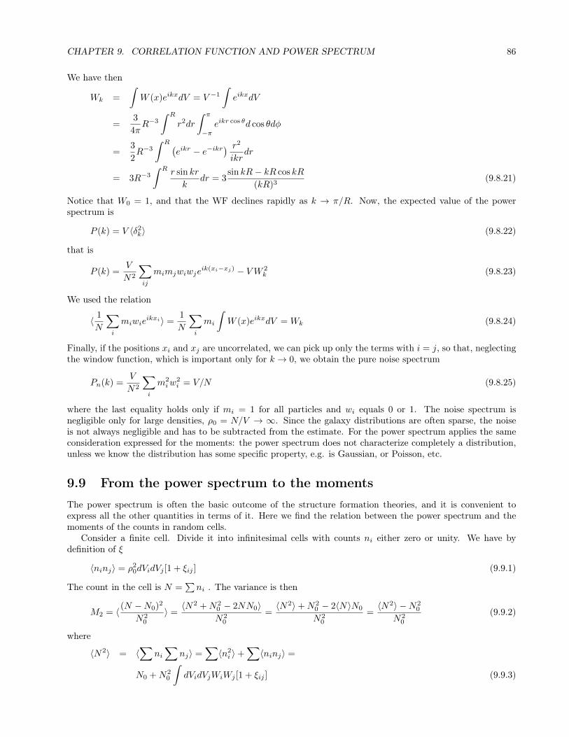
CHAPTER 9. CORRELATION FUNCTION AND POWER SPECTRUM 86
We have then
Wk =
∫W (x)eikxdV = V −1
∫eikxdV
=3
4πR−3
∫ R
r2dr
∫ π
−πeikr cos θd cos θdφ
=3
2R−3
∫ R (eikr − e−ikr
) r2
ikrdr
= 3R−3
∫ R r sin kr
kdr = 3
sin kR− kR cos kR
(kR)3(9.8.21)
Notice that W0 = 1, and that the WF declines rapidly as k → π/R. Now, the expected value of the powerspectrum is
P (k) = V 〈δ2k〉 (9.8.22)
that is
P (k) =V
N2
∑ij
mimjwiwjeik(xi−xj) − VW 2
k (9.8.23)
We used the relation
〈 1
N
∑i
miwieikxi〉 =
1
N
∑i
mi
∫W (x)eikxdV = Wk (9.8.24)
Finally, if the positions xi and xj are uncorrelated, we can pick up only the terms with i = j, so that, neglectingthe window function, which is important only for k → 0, we obtain the pure noise spectrum
Pn(k) =V
N2
∑i
m2iw
2i = V/N (9.8.25)
where the last equality holds only if mi = 1 for all particles and wi equals 0 or 1. The noise spectrum isnegligible only for large densities, ρ0 = N/V → ∞. Since the galaxy distributions are often sparse, the noiseis not always negligible and has to be subtracted from the estimate. For the power spectrum applies the sameconsideration expressed for the moments: the power spectrum does not characterize completely a distribution,unless we know the distribution has some specific property, e.g. is Gaussian, or Poisson, etc.
9.9 From the power spectrum to the momentsThe power spectrum is often the basic outcome of the structure formation theories, and it is convenient toexpress all the other quantities in terms of it. Here we find the relation between the power spectrum and themoments of the counts in random cells.
Consider a finite cell. Divide it into infinitesimal cells with counts ni either zero or unity. We have bydefinition of ξ
〈ninj〉 = ρ20dVidVj [1 + ξij ] (9.9.1)
The count in the cell is N =∑ni . The variance is then
M2 = 〈 (N −N0)2
N20
〉 =〈N2 +N2
0 − 2NN0〉N2
0
=〈N2〉+N2
0 − 2〈N〉N0
N20
=〈N2〉 −N2
0
N20
(9.9.2)
where
〈N2〉 = 〈∑
ni∑
nj〉 =∑〈n2i 〉+
∑〈ninj〉 =
N0 +N20
∫dVidVjWiWj [1 + ξij ] (9.9.3)
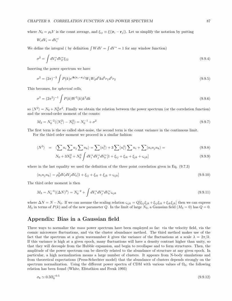
CHAPTER 9. CORRELATION FUNCTION AND POWER SPECTRUM 87
where N0 = ρ0V is the count average, and ξij ≡ ξ(|ri − rj |). Let us simplify the notation by putting
WidVi = dV ∗i
We define the integral ( by definition∫WdV =
∫dV ∗ = 1 for any window function)
σ2 =
∫dV ∗1 dV
∗2 ξ12 (9.9.4)
Inserting the power spectrum we have
σ2 = (2π)−3
∫P (k)eik(r1−r2)W1W2d
3kd3r1d3r2 (9.9.5)
This becomes, for spherical cells,
σ2 = (2π2)−1
∫P (k)W 2(k)k2dk (9.9.6)
so 〈N2〉 = N0 +N20σ
2. Finally we obtain the relation between the power spectrum (or the correlation function)and the second-order moment of the counts:
M2 = N−20 (〈N2
i 〉 −N20 ) = N−1
0 + σ2 (9.9.7)
The first term is the so called shot-noise, the second term is the count variance in the continuous limit.For the third order moment we proceed in a similar fashion:
〈N3〉 = 〈∑
ni∑
nj∑
nk〉 =∑〈n2i 〉+ 3
∑〈n2i 〉∑
ni +∑〈ninjnk〉 = (9.9.8)
N0 + 3N20 +N3
0
∫dV ∗i dV
∗j dV
∗k [1 + ξij + ξik + ξjk + ςijk] (9.9.9)
where in the last equality we used the definition of the three point correlation given in Eq. (9.7.3)
〈ninjnk〉 = ρ30dVidVjdVk[1 + ξij + ξik + ξjk + ςijk] (9.9.10)
The third order moment is then
M3 = N−30 〈(∆N)3〉 = N−2
0 +
∫dV ∗i dV
∗j dV
∗k ςijk (9.9.11)
where ∆N = N −N0. If we can assume the scaling relation ςijk = Q[ξijξjk+ ξijξik+ ξikξjk] then we can expressM3 in terms of P (k) and of the new parameter Q. In the limit of large N0, a Gaussian field (M3 = 0) has Q = 0.
Appendix: Bias in a Gaussian fieldThree ways to normalize the mass power spectrum have been employed so far: via the velocity field, via thecosmic microwave fluctuations, and via the cluster abundance method. The third method makes use of thefact that the spectrum at a given wavenumber k gives the variance of the fluctuations at a scale λ = 2π/k.If this variance is high at a given epoch, many fluctuations will have a density contrast higher than unity, sothat they will decouple from the Hubble expansion, and begin to recollapse and to form structures. Then, theamplitude of the power spectrum can be directly related to the abundance of structure at any given epoch. Inparticular, a high normalization means a large number of clusters. It appears from N-body simulations andfrom theoretical expectations (Press-Schechter model) that the abundance of clusters depends strongly on thespectrum normalization. Using the different power spectra of CDM with various values of Ω0, the followingrelation has been found (White, Efstathiou and Frenk 1993)
σ8 ' 0.5Ω−0.50 (9.9.12)
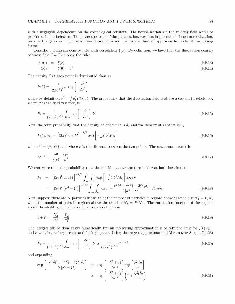
CHAPTER 9. CORRELATION FUNCTION AND POWER SPECTRUM 88
with a negligible dependence on the cosmological constant. The normalization via the velocity field seems toprovide a similar behavior. The power spectrum of the galaxies, however, has in general a different normalization,because the galaxies might be a biased tracer of mass. Let us now find an approximate model of the biasingfactor.
Consider a Gaussian density field with correlation ξ(r). By definition, we have that the fluctuation densitycontrast field δ = δρ/ρ obey the rules
〈δ1δ2〉 = ξ(r) (9.9.13)〈δ2
1〉 = ξ(0) = σ2 (9.9.14)
The density δ at each point is distributed then as
P (δ) =1
(2πσ2)1/2
exp
[− δ2
2σ2
]where by definition σ2 =
∫δ21P (δ)dδ. The probability that the fluctuation field is above a certain threshold νσ,
where σ is the field variance, is
P1 =1
(2πσ2)1/2
∫νσ
exp
[− δ2
2σ2
]dδ (9.9.15)
Now, the joint probability that the density at one point is δ1 and the density at another is δ2,
P (δ1, δ2) =[(2π)
2detM
]−1/2
exp
[−1
2δiδjMij
](9.9.16)
where δi = δ1, δ2 and where r is the distance between the two points. The covariance matrix is
M−1 =σ2 ξ(r)ξ(r) σ2 (9.9.17)
We can write then the probability that the x field is above the threshold ν at both location as
P2 =[(2π)
2detM
]−1/2∫νσ
∫νσ
exp
[−1
2δiδjMij
]dδidδ2
=[(2π)
2(σ4 − ξ2)
]−1/2∫νσ
∫νσ
exp
[−σ
2δ21 + σ2δ2
2 − 2ξδ1δ22 [σ4 − ξ2]
]dδ1dδ2 (9.9.18)
Now, suppose there are N particles in the field; the number of particles in regions above threshold is N1 = P1N ,while the number of pairs in regions above threshold is N2 = P2N
2. The correlation function of the regionsabove threshold is, by definition of correlation function
1 + ξν =N2
N21
=P2
P 21
(9.9.19)
The integral can be done easily numerically, but an interesting approximation is to take the limit for ξ(r) 1and ν 1, i.e. at large scales and for high peaks. Using the large ν approximation (Abramovitz-Stegun 7.1.23)
P1 =1
(2πσ2)1/2
∫νσ
exp
[− δ2
2σ2
]dδ ' 1
(2πν2)1/2
e−ν2/2 (9.9.20)
and expanding
exp
[−σ
2δ21 + σ2δ2
2 − 2ξδ1δ22 [σ4 − ξ2]
]' exp
[−δ
21 + δ2
2
2σ2
]exp
[ξδ1δ2σ4
]' exp
[−δ
21 + δ2
2
2σ2
](1 +
ξδ1δ2σ4
)(9.9.21)

CHAPTER 9. CORRELATION FUNCTION AND POWER SPECTRUM 89
we get
P2
P 21
' 1 +ν2
σ2ξe−ν
2
∫νσ
e−δ21+δ22
2σ2 δ1δ2dδ1dδ2σ4
and finally (Kaiser 1984)
ξν 'ν2
σ2ξ (9.9.22)
This shows that peaks are more correlated than the background density field. This is the same effects oneobserves on mountain ranges: near a peak there is very likely another peak. Eq. (9.9.22) gives some credibilityto the approximation usually made that the galaxy density field is a scale-independent-biased version of themass density field, but it should be noticed that this is expected only for large ν and at large scales, and thatthe whole mechanism relies on the assumption that there is only one object per threshold region.
Eq. (9.9.22) can be applied to clusters. Suppose first we smooth the field on scales of, say, 5 Mpc/h, so thatthe variance σ on such scales is of order unity. It is found observationally that the cluster correlation functionis roughly ten times larger than the galaxy correlation. This would imply a ν ' 3, which is not unreasonable.Notice that some level of biasing is necessary: collapsed object form only where δ > 1.
This concludes the study of the principal estimators of clustering. We can summarize it all by saying that allthe information we have on the large scale distribution can be expressed by the power spectrum P (k) and relatedquantities, and by the higher order parameters like S3, S4. Usually the power spectrum itself is parametrized byan amplitude σ8 and a shape parameter, Γ, so that we can embody our knowledge in four number, σ8,Γ, S3, S4,and a biasing factor if we want to relate observations of different objects to the dark matter distribution. Higherorder moments, or more refined parametrization of the power spectrum are rarely employed, given the relativelysmall amount of data we still have. Of course, we have to be sure that our sample is big enough to include allrelevant wavelengths, otherwise we will find different results in different samples.

Chapter 10
Origin of inflationary perturbations
Quick summary• In general, as we have seen, the perturbations in GR are of three types, scalar, vector and tensor.
• The inflationary quantum mechanism that we are going to discuss will in general excite all three types.However, here again we decide to neglect the vector perturbations since they decay rapidly away.
• The scalar perturbations are complicated by the fact that one needs to perturb at the same time the scalarfield and the metric.
• The tensor perturbations are somehow the easiest to deal with, so we begin with this case.
• We derive the initial spectrum induced by inflation as a function of the slow-rolling parameters.
• Most of the discussion that follows is adapted from Dodelson, Modern Cosmology, Chapter 6.
10.1 From a harmonic oscillator to field quantizationLet us consider a simple harmonic oscillator:
x+ ω2x = 0 (10.1.1)
After quantization, the solution can be formed as a sum of creation/annihilation operators
x = v(ω, t)a+ v∗(ω, t)a† (10.1.2)
where v, v∗are a solution of (10.1.1) and its complex conjugate. Clearly
v(ω, t) ∼ e−iωt (10.1.3)
The operators a, a† obey the commutation relations
[a, a†] ≡ aa† − a†a = 1 (10.1.4)
[a, a] = [a†, a†] = 0 (10.1.5)
and of course the operator a annihilates the vacuum state:
a|0〉 = 0 (10.1.6)
These relations imply
[x,p] = i (10.1.7)
90
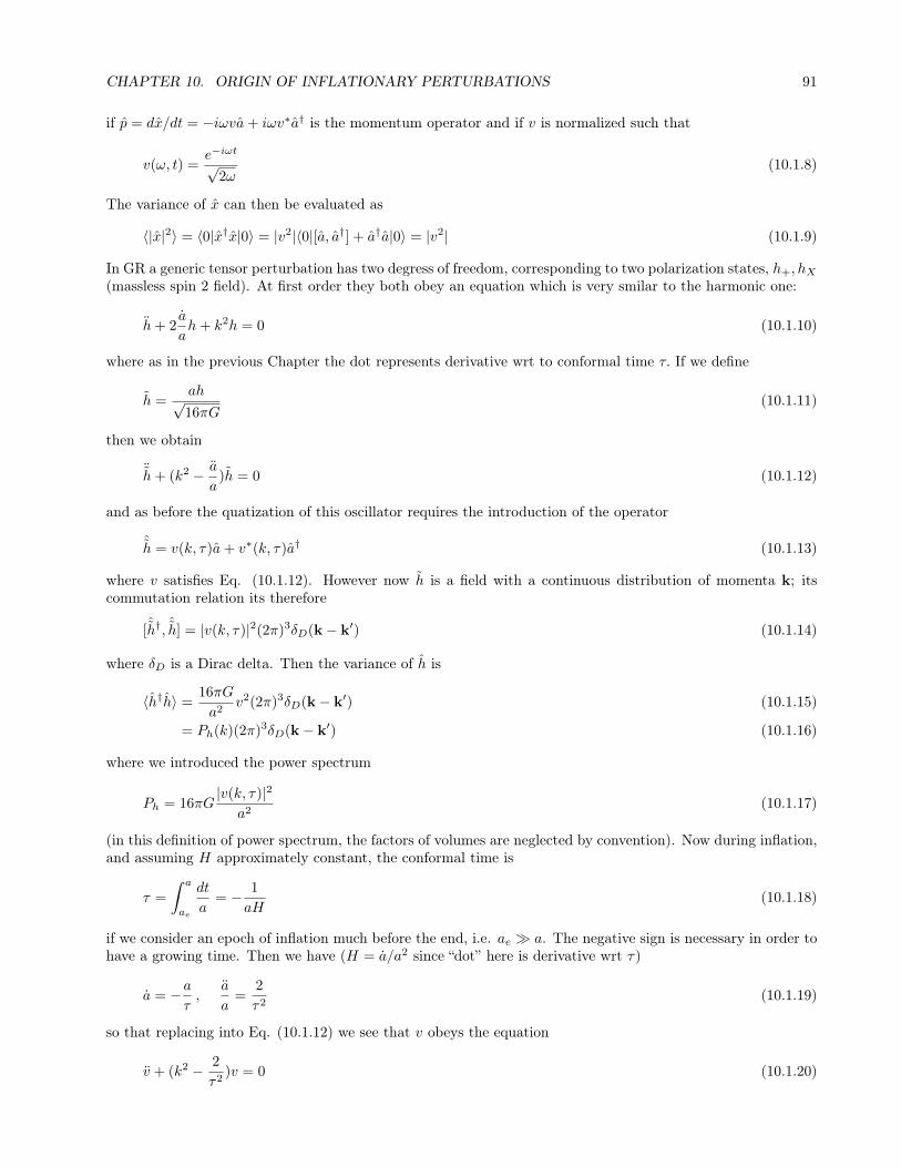
CHAPTER 10. ORIGIN OF INFLATIONARY PERTURBATIONS 91
if p = dx/dt = −iωva+ iωv∗a† is the momentum operator and if v is normalized such that
v(ω, t) =e−iωt√
2ω(10.1.8)
The variance of x can then be evaluated as
〈|x|2〉 = 〈0|x†x|0〉 = |v2|〈0|[a, a†] + a†a|0〉 = |v2| (10.1.9)
In GR a generic tensor perturbation has two degress of freedom, corresponding to two polarization states, h+, hX(massless spin 2 field). At first order they both obey an equation which is very smilar to the harmonic one:
h+ 2a
ah+ k2h = 0 (10.1.10)
where as in the previous Chapter the dot represents derivative wrt to conformal time τ. If we define
h =ah√16πG
(10.1.11)
then we obtain
¨h+ (k2 − a
a)h = 0 (10.1.12)
and as before the quatization of this oscillator requires the introduction of the operator
ˆh = v(k, τ)a+ v∗(k, τ)a† (10.1.13)
where v satisfies Eq. (10.1.12). However now h is a field with a continuous distribution of momenta k; itscommutation relation its therefore
[ˆh†,
ˆh] = |v(k, τ)|2(2π)3δD(k− k′) (10.1.14)
where δD is a Dirac delta. Then the variance of h is
〈h†h〉 =16πG
a2v2(2π)3δD(k− k′) (10.1.15)
= Ph(k)(2π)3δD(k− k′) (10.1.16)
where we introduced the power spectrum
Ph = 16πG|v(k, τ)|2
a2(10.1.17)
(in this definition of power spectrum, the factors of volumes are neglected by convention). Now during inflation,and assuming H approximately constant, the conformal time is
τ =
∫ a
ae
dt
a= − 1
aH(10.1.18)
if we consider an epoch of inflation much before the end, i.e. ae a. The negative sign is necessary in order tohave a growing time. Then we have (H = a/a2 since “dot” here is derivative wrt τ)
a = −aτ,
a
a=
2
τ2(10.1.19)
so that replacing into Eq. (10.1.12) we see that v obeys the equation
v + (k2 − 2
τ2)v = 0 (10.1.20)
CHAPTER 10. ORIGIN OF INFLATIONARY PERTURBATIONS 92
This equation can be solved exactly in terms of Bessel functions. With the initial conditions such that initiallyone has only an outgoing wave, i.e. v ∼ e−ikτ , one gets the exact solution
v =e−ikτ√
2k(1− i
kτ) (10.1.21)
where we employed the same normalization√
2k we have used for the harmonic oscillator. When the waves exitthe horizon during inflation, ie for k|τ | 1, one gets
v = −e−ikτ√
2k
i
kτ(10.1.22)
Ph = 8πGH2
k3(10.1.23)
where we also employed the inflationary solution (10.1.18) aτ = −1/H. This is the expression for the powerspectrum when the waves exit the horizon during inflation. We may expect that the spectrum amplitude doesnot grow as long as the waves remains super-horizon sized, since gravity is effectively frozen on such scales.This spectrum will therefore be the same for large scales when it is finally observed imprinted on the cosmicmicrowave fluctuations.
On the CMB, the observed fluctuations are smaller than ∆T/T ≈ 10−4. The variance in real space oneexpects from a spectrum Ph is (see eq. 9.9.4)
σ2R ≈
∫PhW
2(k)d3k ≈ 8πGH2
∫ ∞kmin
k−3W 2(k,R)d3k (10.1.24)
The last integral is of order unity (it actually has a small logarithmic dependence on the cut-off kmin), soσ2 ≈ GH2, up to order-of-unity factors. The fluctuations due to the GW therefore must be smaller or equalto the observed signal, which means GH2 = G2V = M−4
P E4infl ≤ 10−8 . This gives Einfl ≤ 10−2MP , well
below the Planck scale. If we could measure directly the tensor perturbations on the CMB we could fix theinflationary scale.
The factor 16πG that we inserted in Eq. (10.1.11) can be justified only by writing down the Lagrangianto second order in h. Then one sees that in order to obtain a canonical kinetic term, such a factor becomesnecessary. In turn, a canonical kinetic term is needed to adopt the standard commutation relations.
The slope of the spectrum is defined as
nT − 3 =d logPhd log k
(10.1.25)
so that
nT = 2d logH
d log k(10.1.26)
Now we have
d logH
d log k=
k
H
dH
dk=
k
H
dH
dτ
dτ
dk|k=aH (10.1.27)
The slope depends therefore on how H changes with time, ie on H. Before we assumed that H is approximatelyconstant during inflation, but now this assumption would give zero for nT , so we must work out the first ordercorrection. We define two dimensionless slow rolling parameters:
ε =dH−1
dt= − H
aH2(10.1.28)
δ =1
H
d2φ/dt2
dφ/dt= − a
Hφ(3H
φ
a+ V ′) (10.1.29)

CHAPTER 10. ORIGIN OF INFLATIONARY PERTURBATIONS 93
where the prime is d/dφ (Other choices for the slow-rolling parameters have been introduced, for instance ε1 = ε
and the sequence εn+1 = d ln|εn|dN . Then one has ε2 = 2δ+ 2ε.) Notice that δ = 0 in the m2φ2 case we have seen
before, because we have d2φ/dt2 = 0.The two parameters can be written also dirently in terms of the inflationary potential V . Since we are
interestd only in the first order corrections, we assume now 3H2 ≈ 8πGV and 3H(dφ/dt)+V ′ = 0; differentiatingthe second relation and using the first, we obtain d2φ/dt2 = −dφ/dt(V ′′ + 3dH/dt)/3H . Then one obtains
ε =1
16πG
(V ′
V
)2
(10.1.30)
δ = ε− 1
8πG
V ′′
V(10.1.31)
Then we see from Eq. (10.1.28) that
H = −aH2ε (10.1.32)
Moreover, we have
dτ
dk|k=aH=τ−1 = −d(aH)−1
dk= −d(1/k)
dk=
1
k2(10.1.33)
Finally, we obtain
nT = 2d logH
d log k= −2ε (10.1.34)
This important relation shows that measuring nT is equivalent to measuring ε, i.e. the rate of change of H.
10.2 Scalar perturbationsThe same technique can be applied to the scalar perturbations. Here however one has to first perturb the fieldφ and then relate it to the metric perturbations Φ,Ψ. A detailed treatment can be found in Dodelson, ModernCosmology, Chapter 6. Here we just state the final result. The power spectrum for the potentials Ψ,Φ is
PΨ = PΦ =8πG
9k3
H2
|ε||k=aH (10.2.1)
The most important difference is that now there is the small number ε at the denominator. This means thatwe expect
PS PT (10.2.2)
where S, T denote scalar, tensor perturbations.The slope of the scalar modes is defined as
nS − 4 =d logPΨ
d log k(10.2.3)
This definition implies that the power spectrum of the density contrast δm, which through the Poisson equationis proportional to k2Ψ for sub-horizon modes, is
Pδm ∼ k4PΨ (10.2.4)
and therefore the slope of Pδmwill be exactly nS .To estimate nS we do as before. We have then
nS − 1 =d
d log k[logH2 − log ε] (10.2.5)

CHAPTER 10. ORIGIN OF INFLATIONARY PERTURBATIONS 94
The first term gives −2ε from (10.1.34). The second one can be obtained noting that d/d log k ≈ d/d log a sincek = aH and the variation of H is negligible wrt the variation of a. Then we have from Eq. (10.1.30) and fromdφ/d log a = −V ′/3H2 = −V ′/(8πGV ) that
d log ε
d log k≈ d log ε
d log a=d log ε
dφ
dφ
d log a= − 1
4πG(V ′′
V ′− V ′
V)V ′
V= 2(ε+ δ) (10.2.6)
so that finally
nS = 1− 4ε− 2δ (10.2.7)
Both nS and nT are in general a function of time and therefore, through the relation k = aH, of the scale k.The current estimated value of ns is 0.96± 0.01 (Planck 2015).
The ratio of tensor to scalar spectra can be defined as
rP =PhPΨ
= |9ε| (10.2.8)
but actually it is normally defined as the ratio of the observed spectra, rather than the spectra at horizon exitas here. The observed ratio r turns out to be in simple models of inflation equal to roughly 10ε, but the exactvalue is model- and k-dependent. One very common way to represent the constraints from CMB observationsis to employ the parameter plane τ, nS .
In summary, while the tensor spectrum amplitude measures directly the inflationary energy scale H2 ≈8πGV/3, the scalar spectrum and the spectra slopes measure also the potential derivatives V ′, V ′′ through εand δ.
It is interesting to notice that from the slow roll relation 3H2φ′ + V ′ = 0 (the prime is d/dN) one has
V ′
V=
3H2
V
dφ
dN= 8πG
∆φ
∆N(10.2.9)
and therefore, from (10.1.30),
8πG∆φ
∆N=√
16πGε =
√16πG
r
10(10.2.10)
If, as the experiment BICEP2 (2014) reported, r ≈ 0.2, then
∆φ ≈ 0.14MP∆N (10.2.11)
where MP = (8πG)−2 is the reduced Planck mass. Here ∆N is the number of e-folding elapsed while φ movesby ∆φ. The observational range observed by BICEP2 is of a few e-foldings, eg ∆N ≈ 4, so finally we see thatthe field φ has to move by half a Planck mass or so to produce a value of r close to the observed one. Althoughis not difficult to design by hand models that satisfy this condition, many models that have some theoreticalsupport predict an extremely flat potential and consequently a very small change in φ. In any case, the BICEPresults have been found to be erroneous so at the moment there is no detection of r but only upper limits,r < 0.1 roughly.

Chapter 11
The Cosmic Microwave Background
The cosmic microwave background (CMB) is the oldest cosmological signal we can currently observe. Mappingits fluctuations gives a wealth of accurate information on processes before, during and after the recombination.The recent WMAP and Planck satellites have measured several parameter to percent accuracy by comparingthe temperature and polarization anisotropies to predictions.
Quick summary• The CMB photons have been first captured in 1965 by Penzias and Wilson, definitely confirming the hot
big bang scenario
• The primordial fluctuations created during inflation left their imprint on the photons last scattered atrecombination, i.e. at a redshift of around 1000
• These temperature anisotropies, first observed by the COBE satellite, are due to several physical phenom-ena at recombination time: Sachs-Wolfe effect, baryon oscillation, Silk damping
• Other phenomena are produced along the line of sight: integrated Sachs-Wolfe, lensing, reionization
• Polarization adds another dimension to observations; primordial gravitational waves leave a characteristicimprint on the B-mode polarization
• One of the main problem of CMB observations is the removal of foregrounds due to various non-cosmologicaleffects
11.1 A short history of the CMB researchIn the ’50 scientists started taking into serious consideration the effects of a hot big bang as implied by thediscovery of the cosmic expansion by Hubble. Alpher, Herman, Gamow and others realized that the photons thatinitially dominated the energy density should have been still around after they last scattered when neutral atomsfirst formed at a temperature of a few thousand degrees and at an epoch roughly 350,000 years after the bigbang. They predicted then that a isotropic black-body bath of radiation at around 5K could be detected. Thisindeed occurred in 1965 when Penzias and Wilson discovered by chance a unexplained isotropic 3K radiation,correctly interpreted by Dicke, Peebles and collaborators as the sought-for big bang remnant.
After the full relativistic treatment of linear perturbations developed by Lifshitz and Khalatnikov, andSakharov in the early 60s, Sachs and Wolfe (1966) showed then that the existence of today’s inhomogeneityshould imply some level of inhomogeneities also on the CMB due to the gravitational red- or blueshift inducedby matter perturbations of CMB photons. In subsequent years, Silk, Peebles, Yu and others found out how theinteractions between photon and baryons before and during the recombination process could have imprintedsmall angular scale perturbations due to the propagation of sound waves in the coupled plasma. In the early80s these calculations were extended to take into account dark matter (Silk, Vittorio, Efstathiou, Bond).
95

CHAPTER 11. THE COSMIC MICROWAVE BACKGROUND 96
Figure 11.0.1: Cosmological parameters estimated by the Planck satellite (2015). Fromirsa.ipac.caltech.edu/data/Planck/release_2/ancillary-data/

CHAPTER 11. THE COSMIC MICROWAVE BACKGROUND 97
Nowadays there are several publicly available numerical codes that in a very short time perform the full set ofcalculations in the linear (or even non-linear) regime, including dark matter, baryons, photons, neutrinos, darkenergy, curvature and all possible physical effects, finally producing the predicted CMB and matter clusteringspectra. Among these codes we mention CMBFAST, CMBeasy, CAMB, CLASS.
In the mean time, observations of the CMB failed to find anisotropies until the COBE satellite launchedin 1989 by NASA confirmed the almost perfect black body nature of the radiation spectrum and finally foundsmall fluctuations at angular scales larger than 7 degrees. In the following years many other ground basedobservations tried to increase the resolution to detect the baryon acoustic oscillations. This was first achievedby the Boomerang ballon experiment (de Bernardis), and other similar experiments. The detection of the baryonpeak allowed for the first time to measure the total energy density Ωtot, which turned out to be close to unity aspredicted by inflation. In 2003 the high-resolution WMAP NASA satellite extended the resolution to 10 primesroughly, while Planck (launch 2009), a ESA satellite increased it to roughly 5 primes, also adding more channelsto improve foreground subtraction, and included for the first time sensitive polarization measurements. Planckmeasured several cosmological parameters to a percent accuracy (see Fig. 11.0.1).
11.2 Anisotropies on the cosmic microwave backgroundAt a temperature of roughly 3,000 K, protons combine with electrons to form neutral hydrogen atoms, anddecouple from the radiation. The background radiation we receive today has been emitted therefore roughlywhen the scale factor was ad = 3/3, 000 = 0.001, if today’s temperature is 3K.A black body at this temperaturehas a wavelength peak at λmax ≈ (2.3 · 10−3K ·m)T−1 ≈ 1mm. The redshift of decoupling is zdec ' 1000. Thedistribution of the matter at that epoch is therefore imprinted on the background radiation. There are threemain effects arising from the decoupling surface:
a) The Sachs-Wolfe effect. This occurs because when the photons are emitted from inside a overdensity,they have to climb out the gravitational potential. The SW effect dominates at scales much larger than thehorizon, corresponding to roughly 10
b) The acoustic effect. This occurs because the baryons and the photons perturbations oscillate acousticallywhen they are smaller than their combined Jeans length. We see then fluctuations on the scale of the Jeanslength and higher, corresponding to scales around 10 and smaller.
c) The adiabatic effect. This occurs because if the initial conditions are adiabatic then
δγ =4
3δc. (11.2.1)
All these effects are averaged out on scales much smaller than the last scattering thickness, which is roughly 7Mpc/h. In terms of angular scales, this is
θth = 7/6000(180 · 60/π) = 4′ (11.2.2)
Two effects arise instead along the radiation geodesic to us:d) The integrated SW effect. This occurs whenever the gravitational potential of perturbations is not
constant. Suppose in fact it increases with time. Then, a photon enter at a time when the potential is smallerthan when it exits. Therefore, the blueshift acquired when falling is smaller than the redshift suffered whenexiting, and there is a net redshift contribution. This happens both when the universe is not flat, or when theperturbations do not grow as a, or when the fluctuations become non-linear (Rees-Sciama effect). In the lattercase the effect is on very small scales (ten arcminutes or so).
e) The Sunyaiev-Zeldovich effect. This occurs when the CMB photon crosses a cluster which contains hotplasma. The electrons in the plasma confer energy to the CMB photons, thereby increasing their temperature(inverse Compton scattering). This effect occurs on very small scales, of the order of some arcminutes.
Let us now focus on the first three effects. We can write that the temperature of the photons coming fromthe last scattering surface varies by a ∆T/T due to the sum of these three effects
∆T
T= grav. redshift + adiab.pert.+ acoustic oscill. (11.2.3)
We’ll consider these three effects in turn.
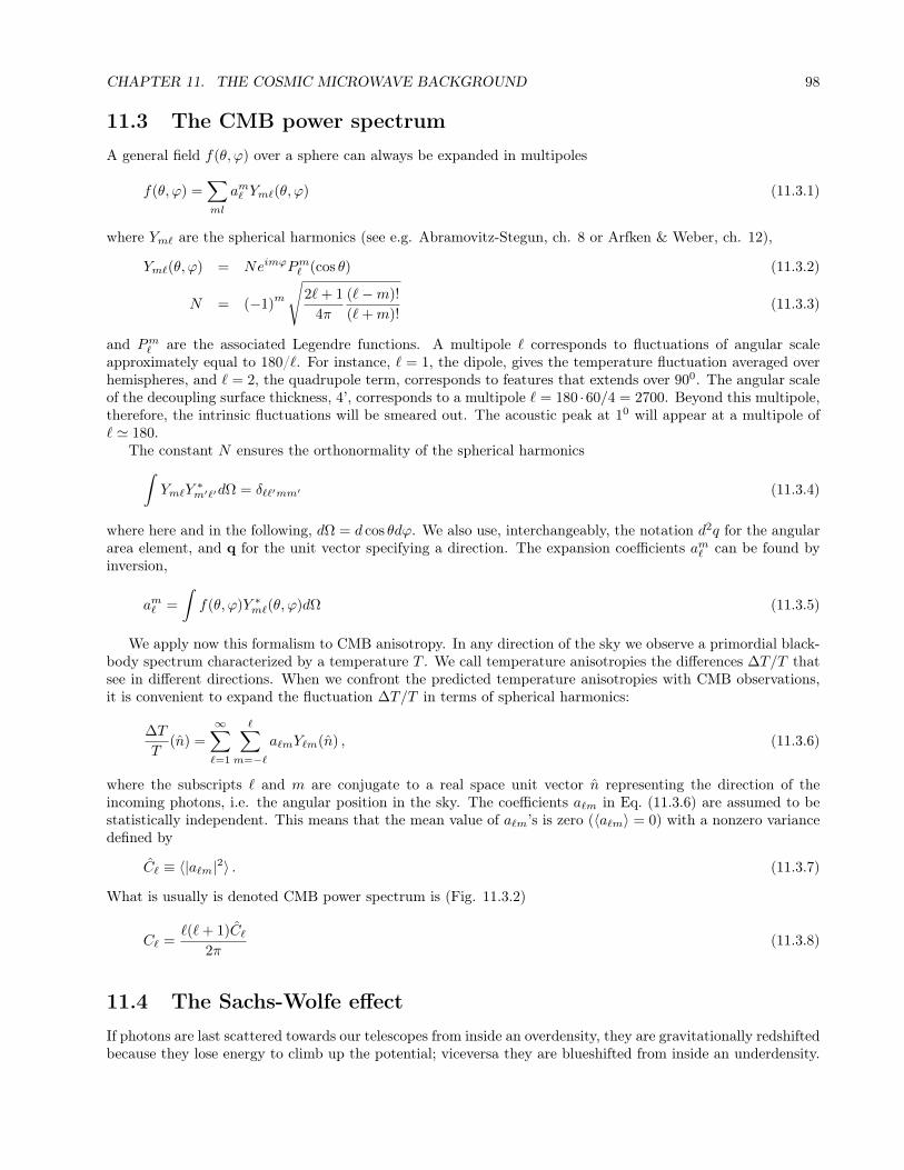
CHAPTER 11. THE COSMIC MICROWAVE BACKGROUND 98
11.3 The CMB power spectrumA general field f(θ, ϕ) over a sphere can always be expanded in multipoles
f(θ, ϕ) =∑ml
am` Ym`(θ, ϕ) (11.3.1)
where Ym` are the spherical harmonics (see e.g. Abramovitz-Stegun, ch. 8 or Arfken & Weber, ch. 12),
Ym`(θ, ϕ) = NeimϕPm` (cos θ) (11.3.2)
N = (−1)m
√2`+ 1
4π
(`−m)!
(`+m)!(11.3.3)
and Pm` are the associated Legendre functions. A multipole ` corresponds to fluctuations of angular scaleapproximately equal to 180/`. For instance, ` = 1, the dipole, gives the temperature fluctuation averaged overhemispheres, and ` = 2, the quadrupole term, corresponds to features that extends over 900. The angular scaleof the decoupling surface thickness, 4’, corresponds to a multipole ` = 180 ·60/4 = 2700. Beyond this multipole,therefore, the intrinsic fluctuations will be smeared out. The acoustic peak at 10 will appear at a multipole of` ' 180.
The constant N ensures the orthonormality of the spherical harmonics∫Ym`Y
∗m′`′dΩ = δ``′mm′ (11.3.4)
where here and in the following, dΩ = d cos θdϕ. We also use, interchangeably, the notation d2q for the angulararea element, and q for the unit vector specifying a direction. The expansion coefficients am` can be found byinversion,
am` =
∫f(θ, ϕ)Y ∗m`(θ, ϕ)dΩ (11.3.5)
We apply now this formalism to CMB anisotropy. In any direction of the sky we observe a primordial black-body spectrum characterized by a temperature T . We call temperature anisotropies the differences ∆T/T thatsee in different directions. When we confront the predicted temperature anisotropies with CMB observations,it is convenient to expand the fluctuation ∆T/T in terms of spherical harmonics:
∆T
T(n) =
∞∑`=1
∑m=−`
a`mY`m(n) , (11.3.6)
where the subscripts ` and m are conjugate to a real space unit vector n representing the direction of theincoming photons, i.e. the angular position in the sky. The coefficients a`m in Eq. (11.3.6) are assumed to bestatistically independent. This means that the mean value of a`m’s is zero (〈a`m〉 = 0) with a nonzero variancedefined by
C` ≡ 〈|a`m|2〉 . (11.3.7)
What is usually is denoted CMB power spectrum is (Fig. 11.3.2)
C` =`(`+ 1)C`
2π(11.3.8)
11.4 The Sachs-Wolfe effectIf photons are last scattered towards our telescopes from inside an overdensity, they are gravitationally redshiftedbecause they lose energy to climb up the potential; viceversa they are blueshifted from inside an underdensity.
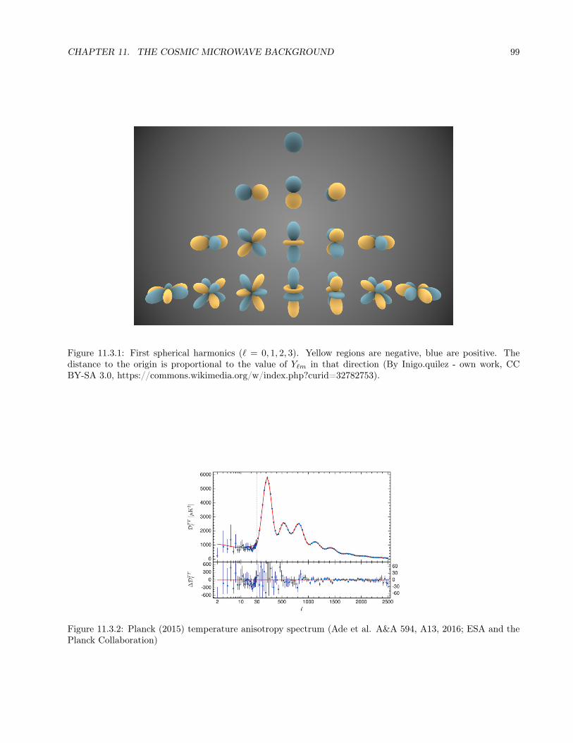
CHAPTER 11. THE COSMIC MICROWAVE BACKGROUND 99
Figure 11.3.1: First spherical harmonics (` = 0, 1, 2, 3). Yellow regions are negative, blue are positive. Thedistance to the origin is proportional to the value of Y`m in that direction (By Inigo.quilez - own work, CCBY-SA 3.0, https://commons.wikimedia.org/w/index.php?curid=32782753).
Figure 11.3.2: Planck (2015) temperature anisotropy spectrum (Ade et al. A&A 594, A13, 2016; ESA and thePlanck Collaboration)
CHAPTER 11. THE COSMIC MICROWAVE BACKGROUND 100
Since we are in a linear regime, the effect must be proportional to the gravitational potential Ψ. It turns outthat the temperature anisotropy is (more details in the Appendix to this chapter)
∆T
T=
Ψ
3(11.4.1)
(for adiabatic perturbations, i.e. when matter and radiation are equally perturbed). Compared to the othereffects, the SW effect is maximal for large perturbations that are still superhorizon at last scattering. Foran initial inflationary power spectrum P (k) ∼ k1 one finds C` ∼ 1/`(` + 1) so that conventionally the powerspectrum is multiplied by `(`+ 1) to render it flat for the SW scales (SW plateau).
The comoving horizon scale at redshift z in a spatially flat (which is a good approximation at large z)matter-dominated universe (neglecting the fact that for z > 3500 the Universe was radiation dominated) is
dcH =
∫ ∞z
dz′
H(z′)=
2
H0
√Ω
(0)m (1 + z)
(11.4.2)
At recombination,r zrec = 1100, we obtain
dcH(zrec) ≈ 180(Ωmh2)−1/2Mpc (11.4.3)
The comoving angular diameter distance d(c)A (zrec) to recombination is expressed as (we now include curvature)
dcA(zrec) =
∫ zrec
0
dz′
H(z′)=
c
H0
√1
Ω(0)K
sinh
(√Ω
(0)K
∫ zdec
0
dz
E(z)
)=
c
H0
1√Ω
(0)m
R , (11.4.4)
where R is the so-called CMB shift parameter defined by
R =
√√√√Ω(0)m
Ω(0)K
sinh
(√Ω
(0)K
∫ zdec
0
dz
E(z)
). (11.4.5)
and in ΛCDM we have E2(z) = Ω(0)m (1 + z)3 + Ω
(0)K (1 + z)2 + (1−Ω
(0)m −Ω
(0)K ). The angular size of the horizon
at recombination is therefore
θH ≈dcH(zrec)
dcA(zrec)≈ (0.0345− 0.05Ω
(0)K )rad ≈ 2 deg (11.4.6)
where the approximation is valid for Ω(0)m = 0.3 and for |Ω(0)
K | < 0.05. corresponding to ` ≈ 90. One can seethat if Ω
(0)K increases, θH decreases, and ` increases (the peak moves to the right, as in Fig. 11.9.1). At larger
scales, where the SW dominates, we expect therefore C` to have an almost flat trend.It is important to remark that the SW effect depends on the total matter content, not just the baryonic one.
In fact, if there were no dark matter, the SW effect would be much smaller than observed or, more precisely,the SW plateau temperature anisotropy would be much lower, with respect to the baryonic peaks, than it isobserved.
Photons can undergo a gravitational shift also during their way to us if they pass through a perturbation thatis evolving with time, so that the opposite shifts when entering and when leaving do not cancel out. This effectis called integrated Sachs-Wolfe (ISW) effect if linear and Rees-Sciama effect if non-linear. The gravitationalpotential is normally constant during the perturbation evolution but not during cosmological transitions, i.e.from radiation to matter (z ≈ 3000) and during any dark energy dominated epoch (z < 1). We expect thereforetwo kinds of ISW, an early and a late one. Since the late effect involves perturbations that are very close to us,and therefore occupy large angular scales, it should affect CMB mostly at very large scales (small `s).
If at the last scattering epoch there are also gravitational waves (generated along with ordinary scalarperturbations during inflation) then these induce also a kind of tensorial SW effect since they act as a oscillatinggravitational potential. Their effect should be much subdominant on the temperature spectrum but might bevisible on the polarization spectrum.

CHAPTER 11. THE COSMIC MICROWAVE BACKGROUND 101
Late ISW
Sachs-Wolfe
Early ISW
Acoustic peaks
Diffusion damping
Figure 11.4.1: The different contributions to the CMB spectrum (Planck 2018, ESA and the Planck Collabora-tion).
Figure 11.4.2: Foregrounds on the CMB spectrum as a function of wavelength (Bennett, C.L., et.al., 2013,ApJS., 208, 20B, WMAP Science Team).
CHAPTER 11. THE COSMIC MICROWAVE BACKGROUND 102
11.5 The baryon acoustic peaksThe next important physical effect on CMB is due to the pressure oscillations in the coupled photon-baryonplasma before last scattering. The sound speed cs is close to the relativistic sound speed c2s = dp/dρ = 1/3.Due to the presence of baryons this speed is however modified as
c2s =dpγ
d(ργ + ρb)=
pγργ + ρb
=43ργ
4ργ + 3ρb=
1
3
1
1 + 3ρb4ργ
=1
3
1
1 + 3Ωb04(1+z)Ωγ0
(11.5.1)
and becomes time-dependent. For instance, at zrec = 1100, since we have Ωb0 = 0.022h−2,Ωγ0 = 2.5 · 10−5h−2,one has
cs,rec ≈ 0.45 (11.5.2)
With this approximation, the sound speed angular size θs ≈ csθH and therefore `s ≈ 200. The oscillations travelwith this speed from big bang (or more exactly from the inflationary epoch) to recombination and thereforeadd a peak of anisotropies at a fixed scale cstrec ≈ 200, 000ly. An exact measurement of this value can find acombination of cs and Ω
(0)K , as in the approximation (11.4.6). This was first obtained by the Boomerang balloon
CMB experiment in 2001. Planck (2015) obtained Ω(0)K = 1− Ω
(0)m − Ω
(0)Λ = 0.01± 0.02.
11.6 The small angular scalesOn smaller scales, the anisotropies are smoothed out because of the finite size of the last scattering “surface”.That is, the photons that escape do not come all from exactly the same redshift but from a region of thickness∆z ≈ 80. Small fluctuations that fit into this thickness scatter photons with a mixture of red- and blue-shifts,which therefore tend to compensate each other in a poissonian way. One can estimate that the diffusion scale,or Silk damping scale, is
θd ≈ 6.4
(Ωmh
2
0.15
)1/4(Ωbh
2
0.02
)−1/2
arcmin (11.6.1)
The CMB power spectrum will be therefore suppressed below this value, corresponding to ` ≈ 2000.
11.7 Reionization and other line-of-sight effects.After recombination, the universe is mostly composed of neutral hydrogen and helium atoms. However whenthe first stars become active, at a redshift of a few, the intergalactic medium reionizes due to the star’s UVemission (see Chap. 17). The free electrons can now re-scatter the CMB photons, effectively smoothing out theCMB angular spectrum. The Thomson optical depth is defined as
τ = c
∫dtneσT (11.7.1)
and is an additional parameter that enters the prediction of the CMB spectrum. Current estimates put thereionization epoch at z ≈ 10.
Photons interact with matter along the line of sight in two other ways. First, they get deviated by thegravitational potentials due to the lensing effect. Second, when they encounter the hot intracluster gas ofgalaxy clusters they are up-scattered by the electrons (Sunyaev-Zel-dovich effect); this distorts the black-bodyspectrum and induce an effective additional blue- or red-shift according to the waveband in which it is observed.
11.8 ForegroundsThe CMB photons get mixed with several other components along their ride to Earth. For instance: emissionfrom dust in the solar system (zodiacal light) and from the Milky Way; galaxy bremmstrahlung; synchrotron andfree-free emission. Fortunately, all these components can be subtracted off the signal because they either comefrom well-known regions of sky or because they have a peculiar frequency spectrum. Observing the microwavesky at different wavebands allow then both to minimize their impact and to subtract it (Fig. 11.4.2).

CHAPTER 11. THE COSMIC MICROWAVE BACKGROUND 103
Figure 11.9.1: Effect of the space curvature on the CMB spectrum (from Sugiyama, PTEP 2014)
Thomsonscatteringonanelectron
Linearpolarization
unpolarizedlight
unpolarizedlight
Figure 11.9.2: Generation of polarization on the CMB (inspired to a drawing by Wayne Hu, back-ground.uchicago.edu/~whu/polar/webversion/polar.html).
11.9 PolarizationThe scattering of photons through electrons and protons introduce also a polarization. If the photons werehomogeneously distributed around the scatterer, the overall polarization would be zero, but since the distributionis not homogeneous, we expect also a net non zero polarization (see Fig. 11.9.2). This has been in fact observedby Planck. The “electric” component of the polarization is tightly related to the temperature anisotropies andis mostly a cross-check of the latter (although additional polarization is induced by lensing). The “magnetic”component can instead be attributed entirely (on large scales) to a very interesting phenomenon, the possibleexistence of gravitational waves on the last scattering surface, generated during inflation. In 2014 the BICEPexperiment announced the detection of this kind of polarization at multipole around ` ≈ 100 but subsequentjoint BICEP-Planck analysis has shown that so far we can only speak of an upper limit to the tensor-to-scalarration r ≤ 0.15 (see definition of r in Ch. 10).
11.10 Boltzmann codesWhen the baryons are inserted into the fluctuation equations, the fluid approximation breaks over. The photonsand the baryons in fact are coupled via the Thomson cross section; on scales larger than the photon mean freepath the full distribution in space and momenta needs to be taken into account (see e.g. Ma & Bertschinger 1995).Publicly available codes (e.g. CMBFAST by Seljak & Zaldarriaga (1995), CAMB by Lewis and collaborators,

CHAPTER 11. THE COSMIC MICROWAVE BACKGROUND 104
CLASS by Lesgourgues and collaborators), do all the numerical computation to a great precision and withhigh speed. At present, the programs can deal with both flat and curved models, and include as componentsphotons, baryons, cold dark matter, and massless and massive neutrinos, some form of dark energy. The maininput parameters are
H0,Ω0,Ωb,ΩΛ, n, h, Tcmb, Nν (11.10.1)
A reionization epoch can also be inserted. The codes include corrections for the gravitational lensing and forreionization. The primordial power spectrum can be parametrized by the slope alone, n. Otherwise, a fullfunctional form of the spectrum can be input. The main output is
P (k), C`,s, Cl,t (11.10.2)
where the subscript t denotes the tensorial perturbations (gravitational waves). Moreover, the power spectrumcan be output at any epoch. The results can be compared to the observations via publicly available MonteCarloroutines.
Appendix: The Sachs-Wolfe effectLet us now considerin more detail the Sachs-Wolfe effect. A photon emitted from inside a fluctuation has toclimb out the gravitational potential, therefore it loses energy and undergoes a gravitational redshift. From GRwe know that the change in wavelength is given by
λobsλem
=1√|g00|
(11.10.3)
In linear perturbation theory, we know that g00 = 1 + 2Ψ where Ψ 1 and therefore
λobsλem
=1√|g00|
≈ 1
1 + ψ≈ 1−Ψ (11.10.4)
and finally
∆λ
λ= −Ψ (11.10.5)
Now, if in a black-body distribution the photons experience a small change in frequency ν ∼ 1/λ, the newblack-body distribution will have a change in temperature
∆T
T=
∆ν
ν= −∆λ
λ= Ψ (11.10.6)
(an increase in frequency produces a proportional increase in temperature, as we see for instance from Wien’slaw, νmax = 5.8 · 10GHzK · T ≈ 170 GHz). Since Ψ is negative for a mass concentration, the temperature issligthly decreased.
At the same time, since there is more matter in this direction, there will be in general also more radiation.In fact, we can assume the adiabatic relation (8.8.4)
δγ =4
3δm
so that, since ργ ∼ T 4,
∆T
T=
1
4δγ =
1
3δm
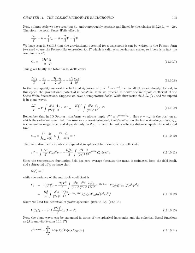
CHAPTER 11. THE COSMIC MICROWAVE BACKGROUND 105
Now, at large scale we have seen that δm and ψ are roughly constant and linked by the relation (8.5.2) δm = −2ψ.Therefore the total Sachs-Wolfe effect is
∆T
T= Ψ +
1
3δm = Ψ− 2
3Ψ =
1
3Ψ
We have seen in Sec.3.3 that the gravitational potential for a wavemode k can be written in the Poisson form(we need to use the Poisson-like expression 8.4.37 which is valid at super-horizon scales, so δ here is in fact thecombination δ∗)
Ψk = −3H2
2
δkk2
(11.10.7)
This gives finally the total Sachs-Wolfe effect
∆TkT
=ψk3
= −H2
2
δkk2
= −H20
2
δk,0k2
(11.10.8)
In the last equality we used the fact that δk grows as a ∼ τ2 ∼ H−2, i.e. in MDE: as we already derived, inthis epoch the gravitational potential is constant. Now we proceed to derive the multipole coefficient of theSachs-Wolfe fluctuations. Suppose we have a temperature Sachs-Wolfe fluctuation field ∆T/T , and we expandit in plane waves,
∆T
T= V
∫d3k
(2π)3
Ψk
3e−ikr = −H
20V
2
∫d3k
(2π)3
δkk2e−ikr (11.10.9)
Remember that in 3D Fourier transforms we always imply eikr ≡ eikr cos θkr . Here r = rem is the position atwhich the radiation is emitted. Because we are considering only the SW effect on the last scattering surface, remis constant in magnitude, and depends only on θ, ϕ. In fact, the last scattering distance equals the conformaltime
rem =
∫ t0
tem
dt
a(t)'∫ t0
0
dt
a(t)= τ (11.10.10)
The fluctuation field can also be expanded in spherical harmonics, with coefficients
am` =
∫∆T
TY ∗m`d
2q = −H20V
2
∫d3k
(2π)3
δ
k2e−ikrY ∗m`(q)d
2q (11.10.11)
Since the temperature fluctuation field has zero average (because the mean is estimated from the field itself,and subtracted off), we have that
〈am` 〉 = 0
while the variance of the multipole coefficient is
C` = 〈(am` )2〉 =
H40V
2
4
∫d3k
(2π)3
d3k′
(2π)3
δkδk′
k2k2′ e−ikr+ik′r′Y ∗m`(q)Ym`(q
′)d2qd2q′
=H4
0
4
∫d3k
(2π)3
P (k)
k4e−ikreikr
′Y ∗m`(q)Ym`(q
′)d2qd2q′ (11.10.12)
where we used the definition of power spectrum given in Eq. (12.4.14)
V 〈δkδk′〉 = P (k)(2π)3
VδD(k − k′) (11.10.13)
Now, the plane waves can be expanded in terms of the spherical harmonics and the spherical Bessel functionsas (Abramovitz-Stegun 10.1.47)
eikr cos θ =
∞∑0
(2`+ 1)i`P`(cos θ)j`(kr) (11.10.14)
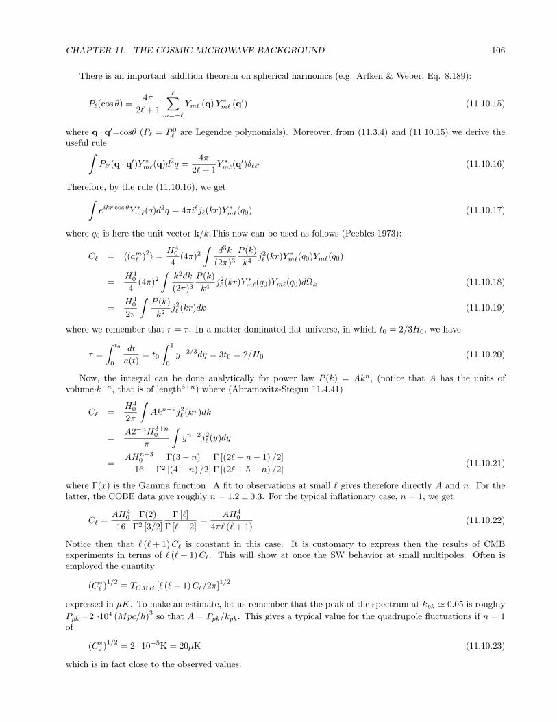
CHAPTER 11. THE COSMIC MICROWAVE BACKGROUND 106
There is an important addition theorem on spherical harmonics (e.g. Arfken & Weber, Eq. 8.189):
P`(cos θ) =4π
2`+ 1
∑m=−`
Ym` (q)Y ∗m` (q′) (11.10.15)
where q · q′=cosθ (P` = P 0` are Legendre polynomials). Moreover, from (11.3.4) and (11.10.15) we derive the
useful rule∫P`′(q · q′)Y ∗m`(q)d2q =
4π
2`+ 1Y ∗m`(q
′)δ``′ (11.10.16)
Therefore, by the rule (11.10.16), we get∫eikr cos θY ∗m`(q)d
2q = 4πi`j`(kr)Y∗m`(q0) (11.10.17)
where q0 is here the unit vector k/k.This now can be used as follows (Peebles 1973):
C` = 〈(am` )2〉 =
H40
4(4π)2
∫d3k
(2π)3
P (k)
k4j2` (kr)Y ∗m`(q0)Ym`(q0)
=H4
0
4(4π)2
∫k2dk
(2π)3
P (k)
k4j2` (kr)Y ∗m`(q0)Ym`(q0)dΩk (11.10.18)
=H4
0
2π
∫P (k)
k2j2` (kr)dk (11.10.19)
where we remember that r = τ . In a matter-dominated flat universe, in which t0 = 2/3H0, we have
τ =
∫ t0
0
dt
a(t)= t0
∫ 1
0
y−2/3dy = 3t0 = 2/H0 (11.10.20)
Now, the integral can be done analytically for power law P (k) = Akn, (notice that A has the units ofvolume·k−n, that is of length3+n) where (Abramovitz-Stegun 11.4.41)
C` =H4
0
2π
∫Akn−2j2
` (kτ)dk
=A2−nH3+n
0
π
∫yn−2j2
` (y)dy
=AHn+3
0
16
Γ(3− n)
Γ2 [(4− n) /2]
Γ [(2`+ n− 1) /2]
Γ [(2`+ 5− n) /2](11.10.21)
where Γ(x) is the Gamma function. A fit to observations at small ` gives therefore directly A and n. For thelatter, the COBE data give roughly n = 1.2± 0.3. For the typical inflationary case, n = 1, we get
C` =AH4
0
16
Γ(2)
Γ2 [3/2]
Γ [`]
Γ [`+ 2]=
AH40
4π` (`+ 1)(11.10.22)
Notice then that ` (`+ 1)C` is constant in this case. It is customary to express then the results of CMBexperiments in terms of ` (`+ 1)C`. This will show at once the SW behavior at small multipoles. Often isemployed the quantity
(C∗` )1/2 ≡ TCMB [` (`+ 1)C`/2π]
1/2
expressed in µK. To make an estimate, let us remember that the peak of the spectrum at kpk ' 0.05 is roughlyPpk =2 ·104 (Mpc/h)
3 so that A = Ppk/kpk. This gives a typical value for the quadrupole fluctuations if n = 1of
(C∗2 )1/2
= 2 · 10−5K = 20µK (11.10.23)
which is in fact close to the observed values.

Chapter 12
The galaxy power spectrum
In Ch. (8) we have seen how to derive the linear matter power spectrum as a function of scale and redshift.What we observe however is the power spectrum of the linear and non-linear galaxy distribution when distancesare measured with the redshift. Its relation to the theoretical prediction is not a straightforward one, as we willsee in this Chapter.
Quick summary• The linear galaxy power spectrum expresses the clustering of galaxies in redshift space
• It is related to theoretical prediction of the matter power spectrum in real space through several corrections(the bias, the redshift distortion) and depends on the growth function
• On small scales, the non-linear effects should also be taken into account
• The baryon oscillations that are prominently visible on the CMB spectrum are also visible as small wiggleson the galaxy power spectrum
• The comparison to observations can constrain several cosmological parameters, from the primordial slopens to Ωm,Ωb, to the dark energy equation of state.
• The Euclid satellite (launch 2021) will measure the power spectrum up to redshift 2 to great precision.
12.1 Large scale structureLet us see now how to link the primordial inflationary spectrum with the present observations of the galaxydistribution. Instead of the spectrum evaluated at horizon reenter, which is different for every scale, we preferto evaluate it at a fixed epoch tF , for instance the decoupling epoch z ≈ 1000. The difference is that at a fixedepoch, the perturbations that are already inside the horizon had the time to grow, contrary to those still outside.Let us consider a perturbation that reenter in MDE when the scale factor was a, and H = (2/3)t−1 = a−3/2H0
(as usual we assume the present value a0 = 1) ; at that epoch, k = aH = aa−3/2H0 = a−1/2H0. Thus aperturbation with wavenumber k reenters when the scale factor was a = (k/H0)−2. This perturbation growsbetween a and an arbitrary instant, say aF , as δk ∼ (aF /a) = (k/kF )2 (since we are in MDE), if kF is the scalethat reenters at aF . Therefore smaller scales reenter the horizon earlier than larger ones and have thereforemore time to grow in amplitude. To conclude, the amplitude of a perturbation of size k−1 has the time to growbetween its reenter and aF by a factor (k/kF )2. Then we have
(δρ/ρ)k(tF ) = (k/kF )2(δρ/ρ)k(tH) , (12.1.1)
and consequently
Pk(tF ) = (k/kF )4Pk(tH) .
107

CHAPTER 12. THE GALAXY POWER SPECTRUM 108
10-4 10-3 10-2 10-1 100
Wavenumber k [hMpc−1]
100
101
102
103
104
Pm(k
)[(h−
1M
pc)
3]
Planck TTPlanck EEPlanck SDSS DR7 LRGBOSS DR9 Ly- forestDES Y1 cosmic shear
Figure 12.1.1: Power spectrum of the large scale structure (at small scales) and of the cosmic microwavebackground (at large scales). (ESA and the Planck Collaboration).
Assuming the inflationary spectrum k−3 of Eq. (10.2.3) it follows that for the scales reentering after equivalence
Pk(tF ) = Ak . Harrison− Zeldovich spectrum (12.1.2)
This scale-invariant spectrum is a remarkable prediction of inflation. During the subsequent evolution, thisinitial spectrum will be modified in a way that depends on the detailed components, e.g. the amount of darkmatter and baryons. Note that we obtained (12.1.2) assuming exponential inflation. If inflation is a powerlaw, the resulting spectrum becomes Pk = Akn, with n ≤ 1. The Planck data of the cosmic background foundn = 0.96± 0.01, in complete agreement with inflation.
We can now predict the observational quantities: the power spectrum and (in the next section) the peculiarvelocity field. Notice that the average of the density contrast vanishes, < δ >= 0, by definition of averagedensity. The simplest non-trivial average quantity that describe the fluctuation field is therefore the dispersionδ, that is the variance < δ2 >. In the Fourier space, the corresponding quantity is the spectrum P (k) = δ2
k.We have seen that the spectrum at horizon crossing goes like k−3, modified in k1 for the perturbations thatreenter in MDE. However, those that are smaller than λeq =13 Mpc h−1, reentering in RDE, do not suffer thiscorrection since as we have seen they do not grow during RDE. In other words, for scales smaller than λeq, thespectrum at horizon crossing coincides with the one at equivalence. For these scales then the behavior remainsk−3. All this means that the inflationary spectrum at a fixed t, P (k) = Akn (with n close to 1) is modifiedduring RDE and MDE by a function T 2(k) such that T ∼ 1 at large scales and T ∼ k−4 at small ones. For thefinal spectrum we have then
P (k) = AknT 2(k) (12.1.3)
where T (k) is called transfer function. This spectrum remains unvaried in slope from equivalence to now: duringthis epoch, in fact, perturbations grow independently of k. A simple form of T 2 that produces the requested

CHAPTER 12. THE GALAXY POWER SPECTRUM 109
behavior is T 2 = 1/[1 + (k/keq)4]. The exact transfer function can be evaluated only numerically, integrating
for every k the perturbation equations. A popular approximation is (Efstathiou, Bond White 1992)
P (k) = AknT (k)2 (12.1.4)
T (k) =[1 +
[ak + (bk)
1.5+ (ck)
2]ν]−1/ν
(12.1.5)
(a, b, c) = (6.4, 3.0, 1.7) Γ−1Mpc/h, ν = 1.13 (12.1.6)Γ = Ωnrh (12.1.7)
where T 2(k) has the correct limit k−4 . The scale at which this limit is approached is kt = Γ = Ωnrh. In a flatmodel with h = 0.5 this is roughly 2π/0.5 Mpc/h = 12.6 Mpc/h, close to the horizon scale at equivalence, as itshould be.
The whole linear treatment fail naturally at very small scales, those that are non-linear and collapsed intogalaxies and clusters. A rough approximation to the linearity scale is 10 Mpch−1.
12.2 The bias factorThe power spectrum we observe is obtained by mapping the position of the galaxies and then performinga Fourier transform of the density contrast. However the power spectrum that is predicted by the linearperturbation theory is the mass power spectrum, not the galaxy one. The density contrast of the galaxiescan be well different from the matter density contrast: for instance, galaxies could form only when the matterdensity is above a certain threshold. The simplest possibility is to assume that the two density contrast areproportional to each other
δg = bδm (12.2.1)
where b is called linear bias factor. In this case obviously
Pg = b2Pm (12.2.2)
Of course the real bias could be a non-linear function of δm, or an average of δm at various locations. In general,the bias factor might depend on space (i.e. on k after Fourier transformation) and time, and also on galaxytype and luminosity. In fact it is often reported that brighter galaxies have a larger bias, perhaps because theyform only on density peaks. The values of b that have been reported so far are always around unity.
12.3 Normalization of the power spectrumSeveral ways to normalize the mass power spectrum have been employed so far: the cosmic microwave fluctua-tions, the cluster abundance, weak lensing.
As we have seen the CMB measures at large scales the Sachs-Wolfe effect, i.e. temperature anisotropiesproportional to the gravitational potential. The amount of anisotropies is then a direct measurement of thepower spectrum at large scales. If we know the shape of the transfer function, measuring the spectrum at largescales fixes its amplitude at all scales and we can estimate the normalization (see Sect. 9.8)
σ28 = (2π2)−1
∫P (k)W 2
8Mpc/h(k)k2dk (12.3.1)
Planck (2015) result assuming ΛCDM is
σ8 = 0.834± 0.03 (12.3.2)
Cluster abundance, along with X-ray mass-temperature relation, is another tool for estimating σ8. In this caseσ8 is strongly degenerate with Ωm but using also the cluster correlation function one can reduce the level ofdegeneracy and measure separately the two parameters. The X-ray survey REFLEX obtained in 2002 the value
σ8 = 0.711± 0.04 (12.3.3)

CHAPTER 12. THE GALAXY POWER SPECTRUM 110
Figure 12.3.1: Planck (2015) constraints on Ωm, σ8 from SZ clusters and from CMB (Ade et al. A&A 594, A13,2016; ESA and the Planck Collaboration).
Clusters detected with the SZ effect by Planck can also give an estimate of σ8 (see Fig. 12.3.1).Finally, in the next chapter we will see that weak lensing can also estimate the amount of clustering regardless
of the galaxy bias, and recent results provide
σ8(Ωm/0.3)0.7 = 0.64± 0.1 (12.3.4)
12.4 The peculiar velocity fieldThe mass power spectrum can be studied also by analyzing the peculiar motion of the galaxies. It is intuitive,in fact, that a more clustered distribution of matter will induce stronger peculiar velocities. The importance ofthis is that the velocity field depends on the total mass distribution, including any unseen component. Let usstart from Eq. (8.6.4). In terms of the time t it becomes
adδ
dt= −ikivi (12.4.1)
Consider now Eq. (8.4.26) for cs = 0:
vi = −Hvi − a2ikiψ (12.4.2)
Expressing the velocity vector by a component parallel and a component orthogonal to the potential gradient(the peculiar acceleration), we see that the orthogonal component (subscript t) obeys the equation
vit = −Hvit (12.4.3)
so that it will decay as a−1. Neglecting therefore this purely rotational component, we can look for solutionsof (12.4.1) in the form vi = F (k)ki. This gives immediately from (12.4.1) the relation between the peculiarvelocity field and the density fluctuations in linear perturbation theory, in the Newtonian regime:
vi = iHaδfki
k2(12.4.4)
where
f =a
δ
dδ
da(12.4.5)

CHAPTER 12. THE GALAXY POWER SPECTRUM 111
is a function that expresses the growth rate of the fluctuations; for a flat universe in MDE we have seen thatδ ∼ a and f = 1. A good approximation for a model with matter parameter Ωm(t), as we have seen in Sec. 8.8, is
f = Ωγm (12.4.6)
with γ ≈ 0.55 and, for ΛCDM,
Ωm(z) =Ωm0(1 + z)3
Ωm0(1 + z)3 + 1− Ωm0(12.4.7)
Let us consider now the present epoch. We put then a = a0 = 1 and H = H0,
v = iH0fδkkk2
(12.4.8)
The peculiar velocity at location x is
v(x) = iH0fV
(2π)3
∫δk
kk2eikrd3k (12.4.9)
and the average in a volume of radius R is
vR = iH0fV
(2π)3VR
∫δk
kk2eikrW (r)d3kd3r = iH0f
V
(2π)3
∫δk
kk2W (kR)d3k (12.4.10)
where W (kR) is the Fourier transform of the window function, defined as
W (kR) =1
VR
∫W (x)eikxd3x
Therefore, the average of the square of the velocity is
〈v2〉R = H20f
2 V 2
(2π)6
∫δkδk′
kk2
k′
k′2W (k′R)W (kR)d3kd3k′ (12.4.11)
=H2
0f2
(2π)3
∫P (k)δD(k − k′) k
k2
k′
k′2W (k′R)W (kR)d3kd3k′ (12.4.12)
=H2
0f2
2π2
∫P (k)W 2(kR)dk (12.4.13)
where in the last integral we integrated over the solid angle 4π and we used the definitions (see 9.8)
V < δkδk′ > =(2π)3
VP (k)δD(k − k′)∫
δD(k − k′)d3k = 1 (12.4.14)
The square root of < v2 >R is called bulk flow, that is the magnitude of the peculiar flow on the scale R.Estimates of the bulk flow can be used then to constrain or normalize the mass power spectrum (see e.g. Lauer& Postman 1996). On the other hand, independent measures of P (k) and 〈v2〉R can give f2 ' Ω1.2
0 and thusΩ0. However, since what we can measure is actually the galaxy power spectrum, assuming a simple biasingPg(k) = b2P (k) we can constrain only the combination β = Ω0.6
m /b.
12.5 The redshift distortionThe galaxy distances we measure are mostly obtained through their redshift. The redshift however includesthe peculiar velocity of the galaxies themselves, so that there is an error in the distances we assign to galaxies.On very small scales the peculiar velocity of a galaxy is more or less randomly oriented, so that the error in
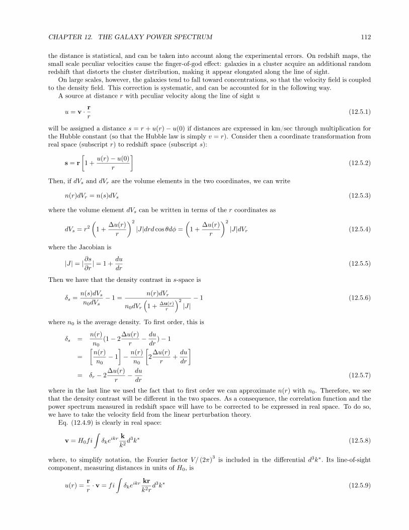
CHAPTER 12. THE GALAXY POWER SPECTRUM 112
the distance is statistical, and can be taken into account along the experimental errors. On redshift maps, thesmall scale peculiar velocities cause the finger-of-god effect: galaxies in a cluster acquire an additional randomredshift that distorts the cluster distribution, making it appear elongated along the line of sight.
On large scales, however, the galaxies tend to fall toward concentrations, so that the velocity field is coupledto the density field. This correction is systematic, and can be accounted for in the following way.
A source at distance r with peculiar velocity along the line of sight u
u = v · rr
(12.5.1)
will be assigned a distance s = r + u(r) − u(0) if distances are expressed in km/sec through multiplication forthe Hubble constant (so that the Hubble law is simply v = r). Consider then a coordinate transformation fromreal space (subscript r) to redshift space (subscript s):
s = r[1 +
u(r)− u(0)
r
](12.5.2)
Then, if dVs and dVr are the volume elements in the two coordinates, we can write
n(r)dVr = n(s)dVs (12.5.3)
where the volume element dVs can be written in terms of the r coordinates as
dVs = r2
(1 +
∆u(r)
r
)2
|J |drd cos θdφ =
(1 +
∆u(r)
r
)2
|J |dVr (12.5.4)
where the Jacobian is
|J | = |∂s∂r| = 1 +
du
dr(12.5.5)
Then we have that the density contrast in s-space is
δs =n(s)dVsn0dVs
− 1 =n(r)dVr
n0dVr
(1 + ∆u(r)
r
)2
|J |− 1 (12.5.6)
where n0 is the average density. To first order, this is
δs =n(r)
n0(1− 2
∆u(r)
r− du
dr)− 1
=
[n(r)
n0− 1
]− n(r)
n0
[2
∆u(r)
r+du
dr
]= δr − 2
∆u(r)
r− du
dr(12.5.7)
where in the last line we used the fact that to first order we can approximate n(r) with n0. Therefore, we seethat the density contrast will be different in the two spaces. As a consequence, the correlation function and thepower spectrum measured in redshift space will have to be corrected to be expressed in real space. To do so,we have to take the velocity field from the linear perturbation theory.
Eq. (12.4.9) is clearly in real space:
v = H0fi
∫δke
ikr kk2d3k∗ (12.5.8)
where, to simplify notation, the Fourier factor V/ (2π)3 is included in the differential d3k∗. Its line-of-sight
component, measuring distances in units of H0, is
u(r) =rr· v = fi
∫δke
ikr krk2r
d3k∗ (12.5.9)
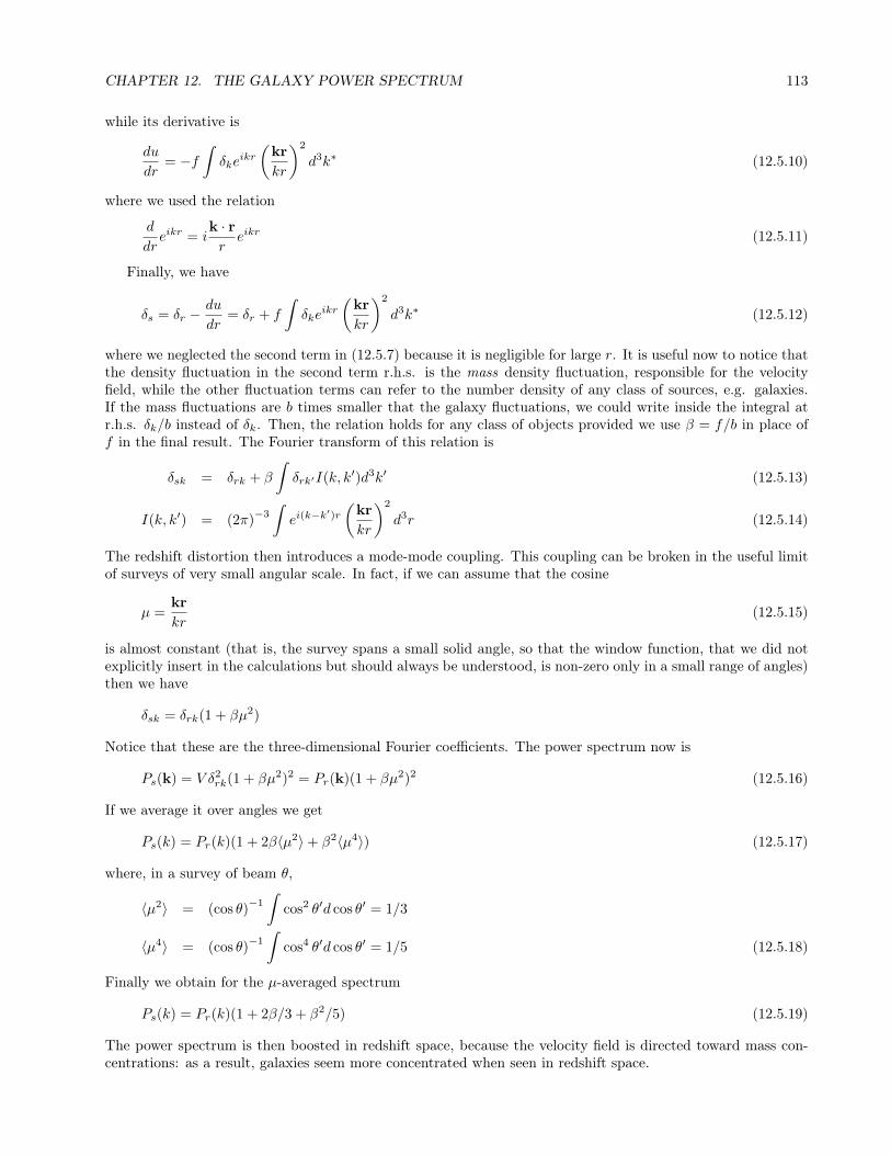
CHAPTER 12. THE GALAXY POWER SPECTRUM 113
while its derivative is
du
dr= −f
∫δke
ikr
(krkr
)2
d3k∗ (12.5.10)
where we used the relation
d
dreikr = i
k · rreikr (12.5.11)
Finally, we have
δs = δr −du
dr= δr + f
∫δke
ikr
(krkr
)2
d3k∗ (12.5.12)
where we neglected the second term in (12.5.7) because it is negligible for large r. It is useful now to notice thatthe density fluctuation in the second term r.h.s. is the mass density fluctuation, responsible for the velocityfield, while the other fluctuation terms can refer to the number density of any class of sources, e.g. galaxies.If the mass fluctuations are b times smaller that the galaxy fluctuations, we could write inside the integral atr.h.s. δk/b instead of δk. Then, the relation holds for any class of objects provided we use β = f/b in place off in the final result. The Fourier transform of this relation is
δsk = δrk + β
∫δrk′I(k, k′)d3k′ (12.5.13)
I(k, k′) = (2π)−3∫ei(k−k
′)r
(krkr
)2
d3r (12.5.14)
The redshift distortion then introduces a mode-mode coupling. This coupling can be broken in the useful limitof surveys of very small angular scale. In fact, if we can assume that the cosine
µ =krkr
(12.5.15)
is almost constant (that is, the survey spans a small solid angle, so that the window function, that we did notexplicitly insert in the calculations but should always be understood, is non-zero only in a small range of angles)then we have
δsk = δrk(1 + βµ2)
Notice that these are the three-dimensional Fourier coefficients. The power spectrum now is
Ps(k) = V δ2rk(1 + βµ2)2 = Pr(k)(1 + βµ2)2 (12.5.16)
If we average it over angles we get
Ps(k) = Pr(k)(1 + 2β〈µ2〉+ β2〈µ4〉) (12.5.17)
where, in a survey of beam θ,
〈µ2〉 = (cos θ)−1∫
cos2 θ′d cos θ′ = 1/3
〈µ4〉 = (cos θ)−1∫
cos4 θ′d cos θ′ = 1/5 (12.5.18)
Finally we obtain for the µ-averaged spectrum
Ps(k) = Pr(k)(1 + 2β/3 + β2/5) (12.5.19)
The power spectrum is then boosted in redshift space, because the velocity field is directed toward mass con-centrations: as a result, galaxies seem more concentrated when seen in redshift space.
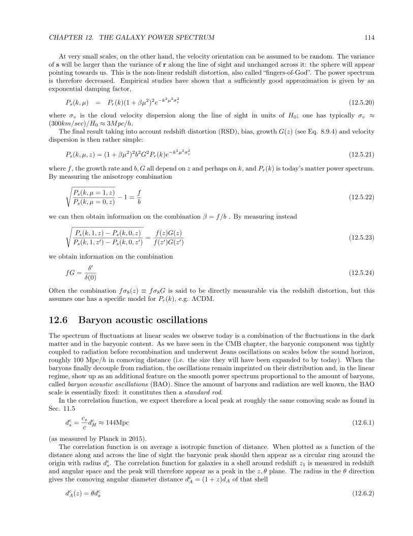
CHAPTER 12. THE GALAXY POWER SPECTRUM 114
At very small scales, on the other hand, the velocity orientation can be assumed to be random. The varianceof s will be larger than the variance of r along the line of sight and unchanged across it: the sphere will appearpointing towards us. This is the non-linear redshift distortion, also called “fingers-of-God”. The power spectrumis therefore decreased. Empirical studies have shown that a sufficiently good approximation is given by anexponential damping factor,
Ps(k, µ) = Pr(k)(1 + βµ2)2e−k2µ2σ2
v (12.5.20)
where σv is the cloud velocity dispersion along the line of sight in units of H0; one has typically σv ≈(300km/sec)/H0 ≈ 3Mpc/h.
The final result taking into account redshift distortion (RSD), bias, growth G(z) (see Eq. 8.9.4) and velocitydispersion is then rather simple:
Ps(k, µ, z) = (1 + βµ2)2b2G2Pr(k)e−k2µ2σ2
v (12.5.21)
where f , the growth rate and b,G all depend on z and perhaps on k, and Pr(k) is today’s matter power spectrum.By measuring the anisotropy combination√
Ps(k, µ = 1, z)
Ps(k, µ = 0, z)− 1 =
f
b(12.5.22)
we can then obtain information on the combination β = f/b . By measuring instead√Ps(k, 1, z)− Ps(k, 0, z)Ps(k, 1, z′)− Ps(k, 0, z′)
=f(z)G(z)
f(z′)G(z′)(12.5.23)
we obtain information on the combination
fG =δ′
δ(0)(12.5.24)
Often the combination fσ8(z) ≡ fσ8G is said to be directly measurable via the redshift distortion, but thisassumes one has a specific model for Pr(k), e.g. ΛCDM.
12.6 Baryon acoustic oscillationsThe spectrum of fluctuations at linear scales we observe today is a combination of the fluctuations in the darkmatter and in the baryonic content. As we have seen in the CMB chapter, the baryonic component was tightlycoupled to radiation before recombination and underwent Jeans oscillations on scales below the sound horizon,roughly 100 Mpc/h in comoving distance (i.e. the size they will have been expanded to by today). When thebaryons finally decouple from radiation, the oscillations remain imprinted on their distribution and, in the linearregime, show up as an additional feature on the smooth power spectrum proportional to the amount of baryons,called baryon acoustic oscillations (BAO). Since the amount of baryons and radiation are well known, the BAOscale is essentially fixed: it constitutes then a standard rod.
In the correlation function, we expect therefore a local peak at roughly the same comoving scale as found inSec. 11.5
dcs =cscdcH ≈ 144Mpc (12.6.1)
(as measured by Planck in 2015).The correlation function is on average a isotropic function of distance. When plotted as a function of the
distance along and across the line of sight the baryonic peak should then appear as a circular ring around theorigin with radius dcs. The correlation function for galaxies in a shell around redshift z1 is measured in redshiftand angular space and the peak will therefore appear as a peak in the z, θ plane. The radius in the θ directiongives the comoving angular diameter distance dcA = (1 + z)dA of that shell
dcA(z) = θdcs (12.6.2)
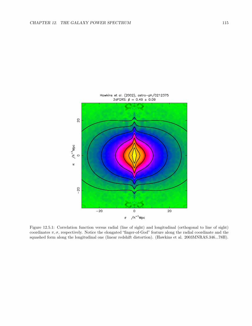
CHAPTER 12. THE GALAXY POWER SPECTRUM 115
Figure 12.5.1: Correlation function versus radial (line of sight) and longitudinal (orthogonal to line of sight)coordinates π, σ, respectively. Notice the elongated “finger-of-God” feature along the radial coordinate and thesquashed form along the longitudinal one (linear redshift distortion). (Hawkins et al. 2003MNRAS.346...78H).

CHAPTER 12. THE GALAXY POWER SPECTRUM 116
Figure 12.6.1: Baryon acoustic peak in a correlation function obtained from MICE, a very large N -bodysimulation. From Fosalba et al. MNRAS 448 (2015), 2987-3000 arXiv:1312.1707.
By estimating the redshift difference ∆z between the two opposite points in the ring one measures instead thedifference of comoving distances along the line of sight:
∆dcA = ∆r =
∫ z1+∆z
0
dz
H(z)−∫ z1
0
dz
H(z)≈ ∆z
H(z)|z1 (12.6.3)
In practice of course the entire ring is fitted by varying the cosmological parameters. Since there are twodirections orthogonal to the line of sight and one along it, one can define a combined distance
DV (z) ≡ [(dcA)2
H(z)∆z]1/3 (12.6.4)
and express the results in terms of DV . Current measurements are however good enough to measure separatelydcA(z) and 1/H(z).
The peak in the correlation function manifests itself also in the power spectrum as the Fourier transform of apeak, namely oscillations at a wavenumber kBAO ≈ 2π/dcA and multiples, appropriately called baryon acousticoscillations (BAO), overimposed to the smooth spectrum, with an amplitude proportional to Ωb.
The baryonic oscillations have been detected for the first time in 2005 with SDSS and 2dFGRS data, obtainingrs
DV (z = 0.35)≈ 0.1± 0.003 (12.6.5)
Subsequent analyses measured the BAO scale to a precision of 2-4%, with results always consistent with con-cordance cosmology.
To go below this precision one needs to take into account small effects that tend to “distort the ring”and smear out the oscillations: the redshift measurement error, the peculiar velocity redshift, the non-linearcorrection to the spectrum. Of course when estimating the cosmological parameters from the power spectrumthe entire shape of the spectrum has to be taken into account, not just the BAO wiggles.
12.7 Non-linear correctionAll we have seen so far is only valid at linear scales where δm 1, i.e. at scales larger than 10 Mpc or so (so infact the k−3 slope is never exactly reached). To measure smaller scales one has two ways: either estimate thespectrum at high redshift or find the non-linear correction.

CHAPTER 12. THE GALAXY POWER SPECTRUM 117
Figure 12.6.2: Baryon acoustic peak observed in the power spectrum of SDSS and BOSS galaxies. The smoothpart of the spectrum has been subtracted. From Anderson et al. 2012, arXiv:1203.6594, Mon. Not. R. Astron.Soc. 427, 3435–3467 (2012).
Figure 12.6.3: Matter power spectrum in linear ΛCDM (black dotted line) and including a simplified halo non-linear correction (q = rs/R and n = d3, green lines), compared with a numerical non-linear spectrum (thickblue dashed line).

CHAPTER 12. THE GALAXY POWER SPECTRUM 118
At redshift zero the ΛCDM spectrum normalization σ equals 0.8 when averaged over spherical cells of radiusR ≈ 8 Mpc/h. At higher redshifts the value of σ8 decreases proportionally to the growth function G. Sincef = d logG/d log a, and putting f ≈ Ωm(a)γone has σ8(z) = G(z)σ8(0) where
G(z) = exp
∫ a
1
f(a′)da′
a′= exp
∫ a
1
Ωγm(a′)da′
a′(12.7.1)
For instance, assuming Ωm0 = 0.3, one has σ8(1) ≈ 0.6 and σ8(3) ≈ 0.3, and therefore the scale of non-linearitymoves to smaller and smaller scales. Intergalactic lumps of neutral hydrogen called Lyman−α clouds along theline of sight of distant quasars absorb part of the quasar radiation and due to different redshifts appear as a“forest” of Lyman−α lines on the quasar’s spectrum (Fig. 12.7.1). Their power spectrum can be calculated upto redshifts of order 4 or even more and provide a window on the linear high−k tail that is otherwise hidden innon-linearities for nearby galaxies.
On smaller scales one should consider non-linear corrections that generally push the power up by even oneorder of magnitude. One rough way of estimating the non-linear correction is to imagine that at small scales theuniverse can be seen as a random collection of identical spherical halos with, for instance, the Navarro-Frenk-White (NFW) profile
ρNFW =ρ0
rrs
(1 + rrs
)2(12.7.2)
where rs is a free scale parameter that has to be fit to each halo. This functional form has been found to be avery good fit to the profiles in N -body simulations. Then one should evaluate the Fourier transform of a singlehalo density contrast in a radius R and volume V = 4πR3/3,
δ1 =4π
V
∫ R
0
(ρNFWρ− 1
)sin(kr)
(kr)r2dr (12.7.3)
=1
V[4π
ρ
∫ R
0
ρNFWsin(kr)
(kr)r2dr − 4π
ρ
∫ R
0
sin(kr)
(kr)r2dr] (12.7.4)
=1
V(WNFW −WTH) (12.7.5)
where ρ is the average density
ρ =4π
V
∫ R
0
ρNFW r2dr (12.7.6)
and then obtain the halo power spectrum as the sum of many random (uncorrelated) halos
Ph(n,R, rs) = NV δ21 = n(WNFW −WTH)2 (12.7.7)
where n is the halo number density. This can be considered a correction to be added to the linear spectrum
PNL = PLIN + Ph (12.7.8)
Some results for PNL are in Fig. (12.6.3). This particular halo correction is very naive and depends on threefree parameters rs, R, n; better non-linear schemes are based on fitting N -body simulations or on higher-orderperturbation theory. We discuss them again in Chap. (14).
12.8 The Euclid satelliteIn 2021 the European Space Agency (with participation from NASA) will launch Euclid, a satellite dedicatedto the study of large scale structure through, primarily, galaxy clustering and weak lensing. The Euclid collab-oration involves 15 countries and over a thousand scientists. The satellite should stay in orbit for five years andscan roughly 15,000 square degrees of sky, that is almost all the sky safely far from the Milky Way disk.
Euclid will have on board a 1,2m telescope with two detectors: a imager and a spectrograph. The imager willcollect the images of two billion galaxies up to redshift 3, while the spectrograph will find the redshift of roughly

CHAPTER 12. THE GALAXY POWER SPECTRUM 119
Figure 12.7.1: Schematic representation of the spectrum of a distant quasar. On the left of the H emissionfrom the quasar itself one sees the forest of Lyman-α absorption lines from clouds on the line of sight at variousredshifts. (From www.nat.vu.nl/~wimu/FundConst-Notes.html, courtesy of Wim Ubachs).
50 million galaxies. The images will be scanned to extract the ellipticity and estimate the shear weak lensingpower spectrum. The galaxy redshifts, along with their angular position in the sky, will provide an accurateestimation of the power spectrum in a volume of 80h−3 cubic Gigaparsecs. This will allow to reconstruct thepower spectrum with an error below 1% over several redshift slices down to z ≈ 2. The cosmological parameterslike ns,Ωm, wDE or even the mass of neutrinos will be estimated to a precision of one per cent or better.
Beside cosmology, Euclid will create immense catalogs of sources (stars, galaxies, clusters, supernovae) thatwill have an impact in almost every field of astronomy. More info on www.euclid-ec.org.

CHAPTER 12. THE GALAXY POWER SPECTRUM 120
Figure 12.8.1: Euclid prediction for various cosmological parameters, using only galaxy clustering. The ellipsesrepresent the confidence regions to 1σ for pairs of parameters, obtained with the Fisher matrix approximation.

Chapter 13
Weak lensing
General relativity shows that a light ray passing at a distance r from a point-like mass M is deflected by anangle
θ =4GM
rc2(13.0.1)
A similar naive calculation in Newtonian physics gives half this result. The light deflection of stars near the limbof the Sun during an eclipse, found by Eddington in 1919, was one of the first evidence in support of GR againstNewtonian gravity. In this chapter we extend this concept to random small fluctuations of the gravitationalpotential.
Quick summary• The image of distant galaxies is magnified and distorted (sheared) by the gravitational potential of struc-
tures along the line of sight
• The magnification is however difficult to detect since galaxies have a very large intrinsic luminosity scatter
• In linear approximation, the distortion is proportional to the second derivative of the potential orthogonalto the trajectory and can be entirely described by a 2× 2 distortion matrix
• The shear correlation or power spectrum is then proportional to the correlation function or power spectrumof matter, no bias has to be taken into account
• Detection of ellipticity has to be extremely precise in order not to introduce artificial anisotropies
• Wide area surveys are necessary to use shear lensing to constrain cosmological parameters
• More details and derivation of several formulae in Dodelson, Modern Cosmology, or Amendola-Tsujikawa,Dark Energy.
13.1 Convergence and shearEq. (13.0.1) can be generalized to give the deflection along a trajectory that passes through a continuousgravitational potential Ψ in the limit of small deviation (weak lensing)
θi = θi + 2
∫ r
0
dr′(1− r′
r)[∇⊥iΨ(r′)] (13.1.1)
(units c = 1) where θi are the angular coordinates of the source (i.e., the unperturbed position) and ∇⊥i isthe gradient orthogonal to the line of sight at position r. The index i runs over 1, 2 to express the two angular
121

CHAPTER 13. WEAK LENSING 122
dimensions on the sky. If the deviation is large then we have some form of strong lensing, for instance doubleimages or arcs. We will not discuss these here.
The angle of deflection itself however cannot be observed since we do not know the “true” direction of theincoming photon, contrary to the case of stars during an eclipse. We can only observe the average statisticaldistortion in nearby light rays, i.e. the derivative
∂θi
∂θj= δij + 2
∫ r
0
dr′(1− r′
r)r′Ψ,ij(r
′) ≡ δij +Dij (13.1.2)
where here θi are the components of the unperturbed direction of the incoming photons and now we havesecond orthogonal derivatives of Ψ (always to be evaluated orthogonally to the line of sight). This equationgives therefore a mapping from the source plane θ to the image plane θ. This defines a distortion matrix for asource (a galaxy) at distance r:
Dij(r) = 2
∫ r
0
dr′(1− r′
r)r′Ψ,ij(r
′) (13.1.3)
This matrix can be written as the sum of a diagonal matrix and a trace-free one,
D =
(−κ− γ1 −γ2
−γ2 −κ+ γ1
)= −κI +
(−γ1 −γ2
−γ2 γ1
)(13.1.4)
where I is the identity matrix and
κ = −∫ r
0
dr′(1− r′
r)r′(Ψ,11 + Ψ,22) (13.1.5)
γ1 = −∫ r
0
dr′(1− r′
r)r′(Ψ,11 −Ψ,22) (13.1.6)
γ2 = −2
∫ r
0
dr′(1− r′
r)r′Ψ,12 (13.1.7)
Here κ is called convergence and γ1,2 shear. If one has a small circular image on the sky, with equationθ2x + θ2
y = r2 and “distorts” it by the transformation θ′i → θi +Dijθj (where i, j = x, y) one obtains at first orderin κ, γ1,2
θ2x(1− 2κ− 2γ1) + θ2
y(1− 2κ+ 2γ1)− 4γ2θxθy = r2 (13.1.8)
or dividing by 1− 2κ (and always linearizing, i.e. for κ, γ1,2 1)
θ2x + θ2
y − 2γ1(θ2x − θ2
y)− 4γ2θxθy = r2(1 + 2κ) (13.1.9)
i.e. the equation of an ellipse that can be decomposed into a new circle of radius r(1 + κ) and an ellipsoidalshear with tilt proportional to γ2 and difference between semimajor axes proportional to γ1. The parametersγ1,2 can indeed be directly used as a measure of the ellipticity of the distortion.
If the galaxy were intrinsically spherical and with a known intrinsic luminosity, then its lensed image wouldshow a change in radius proportional to κ, leading to flux magnification (κ > 0) or demagnification (κ < 0)equal to 1 + 2κ, and a distortion given by γ1,2 and we could directly measure the effect of the potential. Sincehowever galaxies are not spherical nor standard candles, we need to use statistical methods.
Along any given observation beam of finite angular size we see of course not just one but a number ofgalaxies, distributed according to some function n(r). Assuming this distribution is normalized to unity, i.e.∫∞
0n(r)dr = 1, the total distortion matrix can be formed as an average over all the matrices along the line of
sight,
Dij = 2
∫ ∞0
n(r′)dr′∫ r′
0
dr(1− r
r′)rΨ,ij(r) (13.1.10)
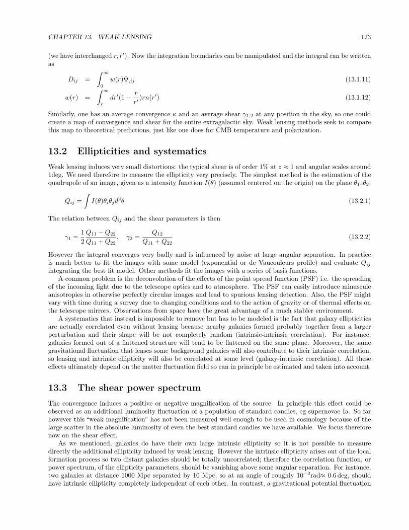
CHAPTER 13. WEAK LENSING 123
(we have interchanged r, r′). Now the integration boundaries can be manipulated and the integral can be writtenas
Dij =
∫ ∞0
w(r)Ψ,ij (13.1.11)
w(r) =
∫ ∞r
dr′(1− r
r′)rn(r′) (13.1.12)
Similarly, one has an average convergence κ and an average shear γ1,2 at any position in the sky, so one couldcreate a map of convergence and shear for the entire extragalactic sky. Weak lensing methods seek to comparethis map to theoretical predictions, just like one does for CMB temperature and polarization.
13.2 Ellipticities and systematicsWeak lensing induces very small distortions: the typical shear is of order 1% at z ≈ 1 and angular scales around1deg. We need therefore to measure the ellipticity very precisely. The simplest method is the estimation of thequadrupole of an image, given as a intensity function I(θ) (assumed centered on the origin) on the plane θ1, θ2:
Qij =
∫I(θ)θiθjd
2θ (13.2.1)
The relation between Qij and the shear parameters is then
γ1 =1
2
Q11 −Q22
Q11 +Q22, γ2 =
Q12
Q11 +Q22(13.2.2)
However the integral converges very badly and is influenced by noise at large angular separation. In practiceis much better to fit the images with some model (exponential or de Vaucouleurs profile) and evaluate Qijintegrating the best fit model. Other methods fit the images with a series of basis functions.
A common problem is the deconvolution of the effects of the point spread function (PSF) i.e. the spreadingof the incoming light due to the telescope optics and to atmosphere. The PSF can easily introduce minusculeanisotropies in otherwise perfectly circular images and lead to spurious lensing detection. Also, the PSF mightvary with time during a survey due to changing conditions and to the action of gravity or of thermal effects onthe telescope mirrors. Observations from space have the great advantage of a much stabler environment.
A systematics that instead is impossible to remove but has to be modeled is the fact that galaxy ellipticitiesare actually correlated even without lensing because nearby galaxies formed probably together from a largerperturbation and their shape will be not completely random (intrinsic-intrinsic correlation). For instance,galaxies formed out of a flattened structure will tend to be flattened on the same plane. Moreover, the samegravitational fluctuation that lenses some background galaxies will also contribute to their intrinsic correlation,so lensing and intrinsic ellipticity will also be correlated at some level (galaxy-intrinsic correlation). All theseeffects ultimately depend on the matter fluctuation field so can in principle be estimated and taken into account.
13.3 The shear power spectrumThe convergence induces a positive or negative magnification of the source. In principle this effect could beobserved as an additional luminosity fluctuation of a population of standard candles, eg supernovae Ia. So farhowever this “weak magnification” has not been measured well enough to be used in cosmology because of thelarge scatter in the absolute luminosity of even the best standard candles we have available. We focus thereforenow on the shear effect.
As we mentioned, galaxies do have their own large intrinsic ellipticity so it is not possible to measuredirectly the additional ellipticity induced by weak lensing. However the intrinsic ellipticity arises out of the localformation process so two distant galaxies should be totally uncorrelated; therefore the correlation function, orpower spectrum, of the ellipticity parameters, should be vanishing above some angular separation. For instance,two galaxies at distance 1000 Mpc separated by 10 Mpc, so at an angle of roughly 10−2rad≈ 0.6 deg, shouldhave intrinsic ellipticity completely independent of each other. In contrast, a gravitational potential fluctuation

CHAPTER 13. WEAK LENSING 124
Figure 13.3.1: Estimates of σ8 and Ωm0 with lensing, BAO and Planck (closed contours). Notice the hint of atension between the weak lensing estimates and Planck. From Planck collab., 2015 (Ade et al. A&A 594, A13,2016); ESA and the Planck Collaboration).
somewhere close to us along the line of sight will lens both galaxies in the same way, inducing a correlation inκ, γ1,2 between different directions.
The calculation of the angular correlation can be performed relatively easily for small angular distances,where the sky can be assumed flat, by applying the Limber projection. At the end of the day, it is clear thatsince κ, γ1,2 are linear functions of Ψ, and Ψ is a linear function of the matter density contrast δm, the finalresult must be that the power spectrum of κ or γ1,2 can be written as a linear function of the matter powerspectrum Pδm(k). In fact one finds (in flat space)
Pκ(`) =9
4
∫ ∞0
dzW (z)2H(z)3Ωm(z)2
(1 + z)4Pδm(
`
r(z)) (13.3.1)
=9
4Ω2m0H
40
∫ ∞0
dz
H(z)W (z)2(1 + z)2Pδm(
`
r(z)) (13.3.2)
where ` = 180 deg /θ is the multipole and
W (z) =
∫ ∞z
dz′
H(z′)
(1− r(z)
r(z′)
)n(z′) (13.3.3)
The galaxy “selection function” n(z) models the number of galaxies n(z)dz at any given redshift z; certainly forsmall z it must go as z2 since dn = n(z)dz ≈ 4πn0z
2dz, but at larger z the galaxies will begin to be too faintto be detected and evolutionary effects will start to take place, so a typical form of n(z) is
n(z) ≈ z2 exp [−(z/z0)α] (13.3.4)
(to be normalized to unity). Very conveniently, one finds that the power spectra of γ1,2 are proportionalto Pκ and do not give additional information. One also finds that the power spectrum of the combinationB = − sin(2φ)γ1 + cos(2φ)γ2 vanishes for any φ as long as the perturbations are induced only by the scalarpart of the metric (i.e. do not include gravitational waves and rotational flows): this part of the weak lensingshear, called magnetic part or B-mode, can then be employed to cross-check the observations. Notice that Pκdepends at small z on Ω2
m0σ28 ; this is the combination to which weak lensing is most sensitive to and often the
observational constraints are reported on the σ8,Ωm0 plane.Finally, one can improve upon Eq. (13.3.1) by considering the shear correlation only among galaxies in a
redshift bin z1, z1 + ∆z, or among two population of galaxies, one in a bin centered at zi and the other at zj :this is called tomographic weak lensing, because it employs also radial information, not just angular correlations.Then given a matter power spectrum Pδm(k) one has
Pκ,ij(`) =9
4
∫ ∞0
dzWi(z)Wj(z)H(z)3Ωm(z)2
(1 + z)4Pδm(
`
r(z)) (13.3.5)
CHAPTER 13. WEAK LENSING 125
where now the window functions Wi include the selection function ni only of the galaxies in the i-th bin.It is important to realize that contrary to the matter power spectrum, here the observed convergence spec-
trum does not need a bias correction, since it depends on the total matter content. Shear weak lensing can givetherefore an absolute normalization of Pδ(k).
13.4 Current resultsShear lensing has first been detected around year 2000 but it took several more years before accurate resultswith systematics under control were produced. In 2011 Lin et al. using SSDS data on 275 square degreesobtained the result
σ8(Ωm/0.3)0.7 = 0.64± 0.1 (13.4.1)
A summary of current results is in Table 3 of Weinberg et al. 2012. A comparison with CMB Planck results isin Fig. (13.3.1). Shear weak lensing will be measured on more than 1/3 of the sky by the Euclid satellite, aswe have seen in Sect. (12.8).

Part III
Galaxies and Clusters
126

Chapter 14
Non-linear perturbations: simplifiedapproaches
Quick summary• Strongly non-linear fluctuations are difficult to handle and normally one has to employ powerful numerical
simulations
• We first introduce the Zel’dovich approximation, which allows to follow in an almost analytical way theinitial stages of structure formation beyond linearity
• Some more analytical results can be obtained assuming a spherical collapse. On scales of galaxies andclusters, Newtonian physics is sufficient
• Spherical collapse gives a simple but surprisingly accurate expression for the density of collapse and ofvirialization
• Using the so-called Press-Schechter formalism, one can approximately predict the number density ofcollapsed object as a function of their maaa, to be compared to real data or simulations
• In this entire chapter we can safey use Newtonian gravity since we deal with scales well smaller than thehorizon.
14.1 The Zel’dovich approximationSo far we have only investigated linear perturbations, except for a brief comment on Sect. 12.7. Stars, galaxiesand clusters, however, are certainly not linear objects. For instance, the density contrast of a typical clusterof galaxies can be δ > 200. Going from the linear treatment to the non-linear one is however generally verydifficult. Even if some important step forward can be achieved by going to higher order in perturbation theory,ultimately one needs large N-body simulations.
A popular way to make progress in non-linear evolution before ressorting to numerical methods is to adoptthe Zel’dovich approximation. The idea is to follow the movement of particles under the action of gravity untilthey hit each other and create a (fomally) infinite density. This should approximate the behavior of particles ina N-body simulation at least at some early time. Consider two sets of comoving coordinates. One, x0, representsthe coordinates of particles in an unperturbed Universe. Since they are comoving, they do not depend on time.The other, x(t), in a perturbed one. Initially, we perturb the position of each particle by a vector field s, calleddisplacement. Then we assume that at some later time t the position of the particles is given by
x(t) = x0 + g(t)s(x0) (14.1.1)
This means we assume the position at time t only depends on the initial displacement through a time (and notspace) dependent function, still to be defined. The density of the particle at any given time is ρ(x, t) in the
127

CHAPTER 14. NON-LINEAR PERTURBATIONS: SIMPLIFIED APPROACHES 128
perturbed Universe and ρ0(t) in the unperturbed one (which just follow the cosmic expansion, ρ0 ∼ a−3). Sincethe particle number density dn = ρdV must be conserved, we have
ρ(x, t)d3x = ρ0(t)d3x0 (14.1.2)
which implies
ρ(x, t) = ρ0(t)
∣∣∣∣ ∂x∂x0
∣∣∣∣−1
(14.1.3)
Let us assume now, without loss of generality, that the coordinates have been chosen along the direction of theeigenvectors of the deformation tensor
dij ≡ −∂si∂x0,j
(14.1.4)
In this case dij is diagonal and therefore∣∣∣∣ ∂x∂x0
∣∣∣∣ =
∣∣∣∣I + g(t)∂s(x0)
∂x0
∣∣∣∣ = |δij − g(t)dij | = (1− gλ1)(1− gλ2)(1− gλ3) (14.1.5)
where I and δij represent the identity matrix and λi are the three eigenvalues of dij (we show below that theeigenvalues are real). This means
ρ(x, t) =ρ0(t)
(1− gλ1)(1− gλ2)(1− gλ3)(14.1.6)
Before we comment on this important expression, let us understand the meaning of g and s. Expanding (14.1.6)for small gλi, we find
ρ(x, t) ≈ ρ0(t)(1 + g(t)(λ1 + λ2 + λ3) = ρ0(t)(1 + g(t)Tr(dij)) (14.1.7)
and therefore
δ(t) ≡ ρ(x, t)− ρ0(t)
ρ0(t)= −g(t)
∂si∂x0,i
= −g(t)∇x0s(x0) (14.1.8)
This expression, being a linearized one, must coincide with the growth law, δ(t) = G(t)δ0, where G(t) is thegrowth function we have evaluated for various cases in Chap. (8). Then we see that we should identify g(t)with G(t) and
−∇x0s(x0) = δ0 (14.1.9)
Now, from the Poisson equation and the Friedmann equation we have
∇2Ψ = 4πρmδ =3
2a2H2ΩmG(t)δ0 (14.1.10)
where the factor a2 arises because we are adopting comoving, rather than physical, coordinates. Then we seethat
δ0 =2
3a2H2ΩmG∇2Ψ (14.1.11)
and therefore
s(x0) = − 2
3a2H2ΩmG∇Ψ (14.1.12)
With this identification of s, the deformation tensor dij is symmetric and therefore its three eigenvalues arereal. Therefore, we have completely specified the prescription (14.1.1): g(t) is the growth factor, and the initial

CHAPTER 14. NON-LINEAR PERTURBATIONS: SIMPLIFIED APPROACHES 129
Figure 14.1.1: Formation of pancakes in a simulation based on the Zel’dovich approximation (from S. Shandarin,arXiv:0912.4520).
displacement field s is essentially the gradient of the gravitational potential, i.e. the force acting on the particles.In this way, one can run a very cheap N -body simulation: first, take the linear power spectrum at some earlyepoch for the model you want to simulate; second, convert the power spectrum for δ into a power sectrum for Ψusing Poisson equation in Fourier space; third, create a real space realization of this spectrum by overimposingsinusoidal oscillations with amplitude given by the spectrum and random phases; fourth, put particles on aregular grid; fifth, evaluate the displacement field by evaluating at every grid point (14.1.12); finally, move theparticles out of their initial grid point by using (14.1.1).
To appreciate strenghts and limits of this technique, let us now come back to Eq. (14.1.6). Since g(t) is agrowing function (we discard the decaying mode, if any), ρ(x, t) will develop a singularity as soon as one thelargest λi is positive. This means that the particle will move primarily along the eigenvector associate to maxλiand form regions of high density on the plane orthogonal to this direction: in other words, particle will tend toform planar structures, called pancakes (or blinis in the original Russian) by Zel’dovich, clearly visible in Fig.(14.1.1). After this singularity, the approximation will no longer be valid. In reality, is already quite surprisingthat the prescription (14.1.1) holds quite well beyond the linear regime!
Once the pancakes have been reached, one might assume that the particles “stick” onto, or oscillate around,the planar regions by friction or some hydrodynamic mechanism, and then continue flowing along the planesreaching the edges (called filaments) and finally slide along the filaments towards halos from which, in turn,galaxies and clusters will form. This is indeed qualitatively what is seen in full N-body simulations. Most ofthe current codes actually exploit the Zel’dovich approximation to speed up the calculations during the earlieststages at z 1.
14.2 Spherical collapsea
After the formation of pancakes, the Zel’dovich approximation is no longer viable, although it can be extendedthrough second-order schemes or ad hoc prescriptions. There is however a way to get, on a first approximationwhich however turns out to be surprisingly accurate, an estimate of an important observable, namely how manyobjects form (i.e., collapse into a virialized structure) for a given mass. This aproximation relies on sphericalityand Gaussianity. The idea is first to find the value of the density contrast in the linear approximation atwhich a spherical perturbation collapse and virializes and then, find the fraction of the Gaussian distributionof perturbations that are above this δ collapse value. This fraction corresponds to the fraction of perturbationsthat form structures for a given mass.
For scales at which Newtonian thery applies, a shell of matter at distance R from the center of a sphericaloverdensity with uniform density ρ moves according to the Newtonian force law
d2R
dt2= −GM(R)
R2= −4
3πGρR , (14.2.1)
where M(R) = 4πρR3/3 is the constant mass inside the shell. Since for pressureless matter the backgroundaAdapted from Amendola & Tsujikawa, Dark Energy. Theory and Observations, CUP 2010.
CHAPTER 14. NON-LINEAR PERTURBATIONS: SIMPLIFIED APPROACHES 130
density scales as ρ0 = (3M(R0)/4π)(R0a(t))−3, where R0 is the initial size of the perturbation, we can definethe density contrast as
δ =
(a(t)R0
R
)3
− 1 , (14.2.2)
inside the shell and δ = 0 outside. The crucial assumption here is that δ is a step, or top-hat, function, whichallows in fact to cancel all spatial derivatives. Replacing R with δ, the equation for δ in our time variable N isthen:
δ′′ +
(1 +H′
H
)δ′ − 3
2Ωmδ =
4
3
δ′2
1 + δ+
3
2Ωmδ
2 . (14.2.3)
Multyiplying Eq. (14.2.1) on both sides by 2dR/dt the equation can be integrated once as(dR
dt
)2
=2GM
R− C , (14.2.4)
where C is an integration constant. This is the cycloid equation, whose solution for C > 0 can be givenparametrically as R = GM(1− cos τ)/C and t = GM(τ − sin τ)/C3/2 where τ ∈ (0, 2π). Substituting in δ andputting a(t) = a0(t/t0)2/3 we obtain in the Einstein-de Sitter case:
δ =9
2
(τ − sin τ)2
(1− cos τ)3− 1 , (14.2.5)
δL =3
5
[3
4(τ − sin τ)
]2/3
, (14.2.6)
where δL (> 0) is the solution of the linearized equation, i.e. the left-hand-side of Eq. (14.2.3). Note thatδ(τ = 0) = 0. It is convenient to use δL as a bookkeeping device: we express the behavior of δ as a function ofδL instead of the parameter τ . A similar solution exists for an underdensity δL < 0. We have assumed a constantmass M(R): this implies that our analysis is valid only until shell-crossing occurs. As one expects, the radius Rfirst increases (a small perturbation expands with the cosmological expansion), reaches a turnaround point andthen decreases to zero (the perturbation collapses under its own gravity). The final singular phase is of courseunphysical because the dust assumption will fail at some high density, non-radial fluctuations will develop andeven the dark matter collisionless component will undergo the so-called “violent relaxation” mechanism and willset into virial equilibrium.
The main result we get from this model is the critical or collapse value δcoll of the linear fluctuation δLthat is reached at the time of collapse. This quantity is of cosmological relevance because it is used in thePress-Schechter theory [?, ?] as a first approximation to the epoch of galaxy formation and to calculate theabundance of collapsed objects, as we will discuss below. It can be seen from Eq. (14.2.6) that when τ = 0 theperturbations are zero, then δ reaches a turnaround at τ = π (for which δT ≡ δ(π) = (3π/4)2 − 1 ≈ 4.6 andδL ≈ 1.063) and finally for τ = 2π the overdensity δ (but of course not δL) becomes singular. This singularityoccurs when
δL = δcoll = (3/5)(3π/2)2/3 ≈ 1.686 , (14.2.7)
and it takes exactly twice as much time as for the turnaround. Notice that this value is independent of time: aspherical perturbation in the Einstein-de Sitter universe collapses to a singularity whenever the linear densitycontrast equals 1.686. For other models, however, δcoll depends on time. An approximation for dark energywith constant wDE in flat space is (Weinberg and Kamionkowski, MNRAS 341, 2003, 251)
δcoll(z) = 1.686 [1 + α(wDE) log10 Ωm(z)] , (14.2.8)α(wDE) = 0.353w4
DE + 1.044w3DE + 1.128w2
DE + 0.555wDE + 0.131 . (14.2.9)
One can define other phenomenologically interesting epochs that are sometimes used: the epoch of non-linearity (δ = 1, corresponding to δL ≈ 0.57) and the epoch of expected virialization. The latter is defined to

CHAPTER 14. NON-LINEAR PERTURBATIONS: SIMPLIFIED APPROACHES 131
correspond to the instant in which the kinetic energy K is related to the gravitational potential energy U bythe condition
K =R
2
∂U
∂R. (14.2.10)
However, it is by no means obvious that this condition is enough to realize virialization, especially when darkenergy is present. For an inverse-power potential (U ∝ −1/R), the virialization implies K = −U/2. The radiusand the density of the perturbation at virialization can be calculated by assuming conservation of energy atturnaround (when the kinetic energy vanishes; subscript T ) and at a virialization epoch tV when the kineticenergy satisfies KV = −UV /2, i.e.
UT = UV +KV = UV /2 . (14.2.11)
Since for a uniform sphere U = −3GM/5R (and remembering once again we are assuming M = constant),we obtain the relation RV = RT /2. Hence the virialized radius is half the turnaround radius. The density insidethis radius turns out to be δV ≈ 178 and the epoch of this occurrence is very close to the final collapse time. Anumerical fit for wDE = constant models in flat space gives (Weinberg and Kamionkowski, MNRAS 341, 2003,251)
δV ≈ 178[1 + b1θb2(z)] , (14.2.12)
θ =1− Ωm(z)
Ωm(z), (14.2.13)
b1 = 0.399− 1.309(|wDE|0.426 − 1) , (14.2.14)b2 = 0.941− 0.205(|wDE|0.938 − 1) , (14.2.15)
if z is the collapse redshift.It is difficult to go much beyond this kind of phenomenological parametrization. A full understanding of
non-linear physics in dark energy would require extensive N -body simulations coupled to lattice simulations ofscalar fields, a technical feat which is still largely to be explored.
14.3 The mass function of collapsed objectsb
The main reason why it is worthwhile to discuss the abstract phenomenon as a “spherical collapse” is thatthe critical value δcoll and the virial radius RV (or rather the mass contained within that radius) enter thePress-Schecther (PS) formula for the abundance of virialized objects. The main idea behind the PS formula isthat we can estimate the number of collapsed objects formed in a random Gaussian field by simply counting atany given time how many regions have an overdensity above the collapse threshold given by δcoll.
Suppose at some redshift z we smooth a random Gaussian field of density fluctuations over cells of radiusR, each containing on average the mass M = 4πR3ρ/3 with ρ(z) the background density. Since the smoothingis a linear operation, if the field is Gaussian then also the density contrast δ in the cells will be distributedas a Gaussian probability distribution function with variance σ2
M (z). Suppose that all the cells with δ > δcoll
undergo collapse and virialization. The fraction of collapsed regions (i.e. the fraction of space containing objectsof mass larger than M) will be then
p(M, z)|δ>δcoll=
1
σM (z)√
2π
∫ ∞δcoll
exp
(− δ2
M
2σ2M (z)
)dδM =
1
2erfc
(δcoll√
2σM (z)
), (14.3.1)
where erfc(x) is the error function. The fraction containing objects of mass within the range [M,M + dM ] isgiven by
dp(M, z) =
∣∣∣∣∂p(M, z)|δ>δcoll
∂M
∣∣∣∣ dM . (14.3.2)
Remember that in general the threshold δcoll depends on z. Although the boxes with δ > δcoll are certainlynot in the linear regime, the idea is to use the linear regime to estimate the fraction of collapsed regions. We
bAdapted from Amendola & Tsujikawa, Dark Energy. Theory and Observations, CUP 2010.

CHAPTER 14. NON-LINEAR PERTURBATIONS: SIMPLIFIED APPROACHES 132
are then implicitly assuming that the variance σM (z) is in the linear regime (σM 1) and therefore that it canbe calculated from Eq. (9.9.6) with the linear spectrum at any redshift. By using the growth function D(z) wehave σM (z) = D(z)σM (0).
Now, suppose in a volume V we find N collapsed objects, each occupying a volume VM = M/ρ. Then bydefinition the volume occupied collectively by the N objects is the fraction dp of V , i.e.
NVM = V dp , (14.3.3)
and therefore the number density dn of collapsed halos with mass in the dM range (the mass function) will be
dn =N
V=
dp
VM=
ρ
M
∣∣∣∣∂p(M, z)|δ>δcoll
∂M
∣∣∣∣ dM =
√2
π
ρ
M2
δcoll
σM
∣∣∣∣d lnσMd lnM
∣∣∣∣ e−δ2coll/(2σ
2M )dM . (14.3.4)
The extra factor of two that we have inserted in the last step is required because we want all the masses to endup in some object, so that we impose the condition
V
∫ ∞0
(dn
dM
)dM = 1 . (14.3.5)
This factor-of-2 adjustment can be justified with a random walk analysis of fluctuations. In any case, one findsit necessary to fit N -body simulations. Sometimes the number density n(M, z) is taken to be the comovingnumber density (i.e. is multiplied by a3): in this case also ρ should be identified with the comoving backgrounddensity.
Equivalently, Eq. (14.3.4) is sometimes written as
M
ρ
∣∣∣∣ dn
d lnσM
∣∣∣∣ = f(σM , z) , (14.3.6)
where all the cosmological information is contained in the function
f(σM , z) =
√2
π
δcoll
σMe−δ
2coll/(2σ
2M ) . (14.3.7)
The number density dn(M, z) can then be “directly” confronted with the observed densities of objects (clusters,galaxies, quasars) at any redshift. The mass M is often taken to be the virial mass of that class of objects.Because of the exponential dependence on δcoll/σM , the PS formula is quite sensitive to the cosmological model(see Fig. 14.3.1).
The simplicity of the PS approach must not hide the fact that it relies on a dangerous extrapolation ofthe linear theory, on the critical assumption of spherical collapse with top-hat filter, on a dubious definition ofvirialization, and on the absence of processes like merging, dissipation, shell crossing. Surprisingly, this shakyfoundation did not prevent the PS formula to prove itself a valuable first approximation to the abundancesobtained through numerical simulations. Not surprisingly, many works have been dedicated to improving theoriginal PS formula by including corrections due to departure from sphericity or merging or by directly fittingto large N -body simulations. A remarkably successful fit is given by (Jenkins et al. MNRAS 321 (2001) 372)
f(σM , z) = 0.315 exp(−|0.61− lnσM (z)|3.8) . (14.3.8)
This fit has been found to hold for a large range of masses, redshifts, and cosmological parameters, includingdark energy with constant or varying wDE .

CHAPTER 14. NON-LINEAR PERTURBATIONS: SIMPLIFIED APPROACHES 133
Figure 14.3.1: The sensitivity of the cluster mass function to cosmological models. Left panel: The cumulativemass function at z = 0 for M > 5 × 10¹⁴ h−1M (M is the solar mass) for three cosmologies, as a functionof σ8; solid line: Ω
(0)m = 1; short–dashed line: Ω
(0)m = 0.3, Ω
(0)Λ = 0.7; long–dashed line: Ω
(0)m = 0.3,Ω
(0)Λ = 0.
The shaded area indicates the observational uncertainty in the determination of the local cluster space density.Right panel: Evolution of n (> M, z) for the same cosmologies and the same mass limit, with σ8 = 0.5 for theΩ
(0)m = 1 case and σ8 = 0.8 for the low-density models. From Rosati, Borgani, Norman, ARAA 40 (2002) 539.

Chapter 15
Measuring mass in stars and galaxies
The matter content of the Universe is measured by first finding the mass contained in stars, then by weighingthe mass of the galaxies by dynamical means. The comparison between the mass in the visible component,stars, dust and gas and the mass obtained by gravitational methods show that most of the mass should be ina component that is not directly visible, dubbed dark matter. In the next chapter we extend these ideas tocluster of galaxies.
Quick summary• The measurement of masses and densities in the universe is a key task of cosmology since energy density
in one of the main ingredients of GR equations
• The basic measure of star masses is through Kepler’s third law applied to binary stars
• Using models of stellar evolution, the mass of a star can be approximately deduced by its luminosity andcolor
• Masses of galaxies can be inferred indirectly using the virial theorem: it turns out that the total gravita-tional mass is larger that the stellar and gas content of many galaxies, pointing to the existence of a largeamount of dark matter in the halos.
15.1 Mass of starsa
The fundamental way to measure star mass is through application of Kepler’s third law to binary stars. If wemeasure the orbital period P in years, the semi-major axis a around the center of mass in A.U. and the massesm1,m2 in solar masses, Kepler’s law becomes very simple
(m1 +m2)P 2 = a3 (15.1.1)
Of course to measure the semi-major axis we must know the distance to the stars. Let us consider first thesimplest case, a visual binary system in which we can directly see both stars. If the stars exhibit very smallDoppler shifts in their spectra, it means that they orbit face-on. In this case, we can measure separately thetwo semi-major axes of the two orbits around the common center of mass. Then we can use the simple relation
m1a1 = m2a2 (15.1.2)
along with (15.1.1) to measure both m1,m2, since a = a1 + a2. If we assume circular orbits, often a very goodapproximation, then we don’t need to assume face-on orbits.
The second case is a spectroscopic binary, in which the two stars are too close to be resolved and we see onlythe varying spectra. If the star eclipse each other it means they orbit edge-on with respect to us. In this case,
aThis section follows closely the treatment of Prof. Bartelmann’s lecture notes.
134

CHAPTER 15. MEASURING MASS IN STARS AND GALAXIES 135
we can measure by Doppler shift their highest velocity when they are at highest elongation: with this geometrythe star velocity is directed entirely towards or away from us and we can measure distances from the center ofmass and periods (using the eclipse epochs). So again we have two equations, Kepler 3rd law and the velocityrelation
m1v1 = m2v2 (15.1.3)
and we can close the system.In more general cases, the orbits can take place on a plane with inclination i with respect to us and we can
see only the velocity component along the line of sight, v sin i. The masses will then be known only up to thisfactor.
In this way we can calibrate a number of scaling relations between the main properties of stars, namelymass, luminosity, temperature, density, pressure, radius, age. These relation are obtained by the fundamentalequations of star equilibrium. These are: hydrostatic equilibrium between the pressure gradient and the forceof gravity
1
ρ
dP
dr= −GM
r2(15.1.4)
the conservation of mass
dM
dr= 4πr2ρ (15.1.5)
the conservation of energy
dL
dr= 4πr2ρε (15.1.6)
where ε is the energy production rate per mass. Then there is a fourth relation which expresses how thetemperature changes with r according to the energy transport in the star interior. Assuming pure radiativetransfer (i.e propagation of photons) as in main sequence stars, this equation reads
dT
dr= − 3Lκρ
64πr2σT 3(15.1.7)
where
σ =2π5k4
B
15h3c2 = 5.67 · 10−5 erg
cm2K4(15.1.8)
is Stefan-Boltzmann constant and κ is the opacity of the star. Basing on these equations the evolution of starscan in principle be followed until their death through explosion or passive cooling (see Fig. 15.1.1).
Putting ρ ∼M/R3 the hydrostatic equation gives immediately (here and below “∼” means proportional to)
P ∼ GM2
R4(15.1.9)
and inserting the equation of state of an ideal gas PV = nRT or T ∼ P/ρ, we find
T ∼ M
R(15.1.10)
Assuming κ independent of temperature, Eq. (15.1.7) gives
T 3dT ∼ LMr−5dr (15.1.11)
i.e. L ∼ T 4R4/M or the important relation
L ∼M3 (15.1.12)

CHAPTER 15. MEASURING MASS IN STARS AND GALAXIES 136
Figure 15.1.1: Evolutionary tracks of stars on the Hertzsprung-Russell diagram (courtesy of Jan Rybizki).
when combined with (15.1.10). A power M3.5 gives however a more accurate approximation. Now the lifetimeof a star on the main sequence times the luminosity should be proportional to the star fuel and therefore to itsmass, so
LτMS ∼M (15.1.13)
and therefore
τMS ∼M−2 ∼ L−2/3 (15.1.14)
The total luminosity of a star must also be proportional to its surface area and to T 4, i.e. L ∼ R2T 4. Then bycombining with T ∼M/R and with L ∼M3 one also obtains
T ∼ R, M ∼ R2, τMS ∼ T−1 (15.1.15)
In practice, one evolves a numerical code to estimate precise relations among the various parameters. Themass-luminosity relation
L
L= β
(M
M
)α(15.1.16)
shows an index α that varies from 2 to 4 depending on the star mass range and type and a constant β that isaround unity for masses < 20M. Calibrating these relations with local samples one can estimate the massesof stars by their luminosity.
15.2 Mass of galaxiesIf a star moves in a circular orbit around the center of a spherical galaxy at distance R, then by the equilibriumof centripetal force and gravity one has
v2 =GM
R(15.2.1)
and the mass would be very easily estimated. For the Sun, moving at V ≈ 220 km/sec at a distance of8kpc≈ 2.6 · 1020m, one would get M ≈ 2 · 1041kg i.e. roughly 1011 solar masses, which is a very reasonableestimate. However galaxies do not look spherical and many stars do not have circular orbits.
If one assumes that most of the mass of spiral galaxies is concentrated in the roughly spherical central part(the bulge) then stars outside this region should have as in the previous case a Keplerian velocity
v ∼ r−1/2 (15.2.2)

CHAPTER 15. MEASURING MASS IN STARS AND GALAXIES 137
31
Figure 15.1.2: Rotation curve in NGC3198 and the disk and halo components.
Figure 15.2.1: Rotation curves for many spiral galaxies (Sofue et al. 1999 ApJ, 523, 136S ).
However we observe that the rotation velocity of stars and gas in spirals does not decay as r−1/2 but ratherstays approximately constant up to large distances, eg 30 kpc (see Fig. 15.2.1). The simple sun-like geometryof a central concentration cannot explain this behavior. Spiral galaxies are then modeled as the sum of a smallspherical bulge, an extended flattened disk and a large spherical halo mostly composed of invisible dark matter(Fig. 15.2.2). If the halo density profile goes like ρ ∼ r−2 then one finds v = const. This density profile howeverdoes not converge to a finite mass so it must be truncated or steepened at some large radius.
The comparison of these galaxy models to observations can be summarized in the mass-to-light ratio
Y ≡ M
M·LL
(15.2.3)
Current results vary from Y ≈ 1− 30 for galaxies to Y ≈ 100 for clusters. This is a strong evidence in favor ofthe existence of a large component of dark matter. The ratio depends also on galaxy type, on the radius withinwhich is measured, on the waveband and on various other characteristics of the objects. The value in the solarneighborhood is 2± 1. In a sample of elliptical and lenticulars it has been found
Y = (3.8± 0.14)(σe
200km/sec)0.84±0.07 (15.2.4)
where σe is the line-of-sight velocity dispersion, within an effective radius Re measured as the radius thatcontains half of the total galaxy light.

CHAPTER 15. MEASURING MASS IN STARS AND GALAXIES 138
Figure 15.2.2: Structure of the Milky Way (courtesy of Jan Rybizki).
15.3 Halo profilesAn important outcome of N-body simulations is the observation that the density ρ(r) of dark matter in haloshas a more or less universal form. A lot of discussion about the validity of the cosmological models, and ofthe simulations themselves, centers around the determination of the best fitting halo profiles, and on theircomparison to real galaxies, in particular to their rotation curves. All the halo profiles assume a sphericaldistribution (although halos can have significant deviations from sphericity). It is to be remarked that mostproposed halo profiles are purely phenomenological, i.e. fits to N-body simulation, and have very little theoreticalsupport. An extensive collection of results concerning halo profile can be found in Coe astro-ph/1005.0411.
The most well-known is the Navarro-Frenk-White (NFW) profile
ρ(r) =ρs
(r/rs)(1 + r/rs)2(15.3.1)
which can be applied to dark matter halos from galaxy to clusters. Since it is singular at r = 0, this profileis called a cuspy profile, in contrast with cored profiles for which ρ(r → 0) = ρc. At r = rs, one can see thatρ ∼ r−2, i.e.
s =d log ρ
d log r|r=rs = −2 (15.3.2)
At these scales, therefore, we expect flat rotation curves.The mass inside r is
M(r) = 4π
∫ρ(r)r2dr = 4πρsr
3s( ln(1 + x)− x
1 + x) (15.3.3)
where x = r/rs. Notice that the mass vanishes at r → 0 but slowly diverges at large distances: a cut-off is thennecessary. As we have seen in the section on spherical collapse (14.2), objects virialize when the non-linear densitycontrast is around 178, with a weak dependence on cosmology. This number is often approximated as ∆c = 200.This means the object contains within the virialization radius a density ∆cρcrit, where ρcrit = 3H2/8πG is thecritical density at that epoch. The mass inside the radius of virialization rvir is then
Mvir =4
3π∆cρcritr
3vir (15.3.4)
(also calledM200 to specify the exact value chosen for ∆c) So we can introduce a new combination of parameters,the so-called concentration c
c =rvirrs
(15.3.5)

CHAPTER 15. MEASURING MASS IN STARS AND GALAXIES 139
More in general, the concentration is defined as c = rvir/r−2, where r−2 is the radius at which the slope of ρ(r)is -2, so for NFW r−2 = rs. Then by combining (15.3.3) and (15.3.4) one has
ρsρcrit
=∆c
3
c3
ln(1 + c)− c/(1 + c)(15.3.6)
One could then equivalently characterize the NFW profile either by ρs, rs or by Mvit, c. The value of c canhowever be linked to M200, although with a large scatter. From N-body simulation it appears in fact that thereexists a concentration relation, for instance (Duffy et al. 2008)
c200 ≈ 5.7
(M200
2× 10¹²h−1M
)−0.097
(15.3.7)
Assuming this relation, the NFW profile depends on a single parameter. For instance, for a cluster of M ≈2 ·1014M/h, one has rvir ≈ 1 Mpc/h and rs = rvir/c ≈ 0.3 Mpc/h. The concentration relation can be differentfor more relaxed clusters, and also depends on redshift and on the underlying cosmology, especially on the levelof fluctuations σ8. A recent accurate determination is in Dutton and Maccio’ (2014). When applied to real data(through rotation curves), the concentration relation looks quite less tight than in simulations.
The gravitational potential from a mass profile M(r) is
Ψ = G
∫ r
r0
M(x)
x2dx (15.3.8)
and the velocity of stable circular orbits is
v2 = rdΨ
dr=M(r)
r(15.3.9)
which as expected decreases much slower than the Keplerian law v ∼ 1/r for r > rs (se Fig. 15.3.1).The observed velocities are however to be obtained by the sum of the gravitational potential of dark matter
and baryons. Usually the baryons are modeled as the combination of a roughly spherical bulge, a gaseouscomponent and an extended disk:
Ψ = Ψbulge + Ψgas + Ψdisk + ΨDM (15.3.10)
We can infer the baryonic mass directly from observations, up to unknown multiplicative constants: the mass-to-light ratios for disk and bulge, Yb,d (the gas component is supposed to have a universal mass-to-light ratiothat can be inferred from fundamental principles). These ratios can be estimated from stars near the Sun, butremain quite uncertain when applied to other galaxies, so are better left as free parameters. The Yb,d parametersare O(1) dimensionless numbers that quantify how much bigger or smaller the mass associated to the integratedlight from the bulge or the disk is. For instance, Yb = 0.5 means that for every erg/s of light coming fromthe bulge of a galaxy, one should associate half the mass it would associate in our local environment. So thebaryonic component in the bulge, for instance, contributes by Yb times the gravitational potential we wouldhave inferred had we used the Milky Way local mass-to–light ratio. The total velocity we expect to observe canthen be decomposed into a sum
v2obs = Ybv
2bulge + v2
gas + Ydv2disk + v2
DM (15.3.11)
A galaxy rotation curve can then be fitted quite generally with four free parameters (Yb, Yd,M200, c), or threeif we adopt the concentration relation. If the best fit gives M200 > 0, as it occurs for almost all galaxies wecurrently observe, then we can say we need dark matter.
Many other profiles have been proposed, for instance generalized NFW profiles
ρ(r) =ρs
(r/rs)γ(1 + r/rs)3−γ (15.3.12)
which has the same large r behavior ρ ∼ r−3 but a flexible inner profile, ρ(r → 0) ∼ r−γ . Another one is theEinasto profile
ρ(r) = ρ−2 exp
(− 2
α[(
r
r−2)α − 1]
)(15.3.13)
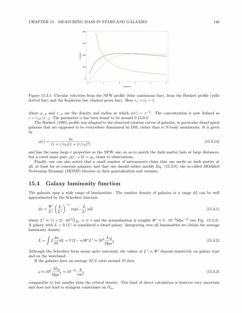
CHAPTER 15. MEASURING MASS IN STARS AND GALAXIES 140
0 1 2 3 4 5
0
100
200
300
400
distance
velocity
Figure 15.3.1: Circular velocities from the NFW profile (blue continuous line), from the Burkert profile (yellodotted line) and the Keplerian law (dashed green line). Here rs = r0 = 1.
where ρ−2 and r−2 are the density and radius at which ρ(r) ∼ r−2. The concentration is now defined asc = rvir/r−2. The parameter α has been found to be around 0.15-0.3.
The Burkert (1995) profile was adapted to the observed rotation curves of galaxies, in particular dwarf spiralgalaxies that are supposed to be everywhere dominated by DM, rather than to N-body simulations. It is givenby
ρ(r) =ρ0
(1 + r/r0)(1 + (r/r0)2)(15.3.14)
and has the same large r properties as the NFW one, so as to match the dark matter halo at large distances,but a cored inner part, ρ(r → 0) = ρ0, closer to observations.
Finally, one can also notice that a small number of astronomers claim that one needs no dark matter atall, at least for as concerns galaxies, and that one should rather modify Eq. (15.3.8), the so-called MOdifiedNewtonian Dynamic (MOND) theories or their generalization and variants.
15.4 Galaxy luminosity functionThe galaxies span a wide range of luminosities. The number density of galaxies in a range dL can be wellapproximated by the Schechter function
dn =Φ∗
L∗
(L
L∗
)−αexp(− L
L∗)dL (15.4.1)
where L∗ ≈ (1 ÷ 2) · 1010L, α ≈ 1 and the normalization is roughly Φ∗ ≈ 5 · 10−3Mpc−3 (see Fig. 15.4.2).A galaxy with L < 0.1L∗ is considered a dwarf galaxy. Integrating over all luminosities we obtain the averageluminosity density
L =
∫Ldn
dLdL = Γ(2− α)Φ∗L∗ ≈ 108 L
Mpc3 (15.4.2)
Although the Schechter form seems quite universal, the values of L∗, α,Φ∗ depend sensitively on galaxy typeand on the waveband.
If the galaxies have an average M/L ratio around 10 then
ρ ≈ 109 MMpc3 ≈ 10−31 g
cm3(15.4.3)
comparable to but smaller than the critical density. This kind of direct calculation is however very uncertainand does not lead to stringent constraints on Ωm.

CHAPTER 15. MEASURING MASS IN STARS AND GALAXIES 141
Figure 15.4.1: Relation between M/L and the velocity dispersion of elliptical and lenticular (S0) galaxies(Cappellari et al. 2006, Mon. Not. R. Astron. Soc. 366, 1126–1150 (2006)).
Figure 15.4.2: Galaxy luminosity function in the 2dFGRS survey, compared with a simulation and fitted by aSchechter function (from Smith 2012, 2012 MNRAS,426,531S ).

Chapter 16
Cosmology with galaxy clusters
Galaxy clusters occupy a special position in cosmology, since they are the largest gravitationally bounded objectin the Universe. They are therefore a bridge between linear scales, where the memory of the initial conditions isstill fully traceable, and the strongly non-linear scales in which other non gravitational phenomena take place.Galaxy clusters can be studied by looking at the dynamics of member galaxies, at the X-ray emission of the hotintra cluster gas, at weak and strong lensing, and at the Sunyaev-Zel’dovich effect on the CMB photons. Wewill discuss some of these topics in this chapter.
16.1 Quick summary• Galaxy clusters are the largest gravitational bounded object on the Universe
• They can be studied by internal dynamics, strong and weak lensing, X-ray emission of the hot intraclustercomponent, Sunyaev-Zel’dovich effect
• All these probes point to a large amount of dark matter, ten times the baryonic component
• Clusters are a direct probe of cosmology also because their number density depend sensitively on pertur-bation growth and on volume measurements
16.2 Mass of clustersGalaxy clusters are groups of hundreds to thousands galaxies within roughly 1 Mpc radius from their center.The closest cluster is Virgo (15 Mpc/h away); the closest rich and regular cluster is Coma (65 Mpc/h). Themost regular among them appear as relatively isolated, almost spherical, groups in equilibrium (i.e. withoutsignificant subclustering neither in space nor in velocity).
There are at least three independent methods to determine the mass of clusters: (i) hydrostatic equilibriumbetween the intra-cluster medium (ICM) and the gravitational potential, (ii) dynamics of member galaxies, and(iii) lensing. We discuss here the first method.
Hydrostatic equilibrium for the ICM gas means that the gradient of the pressure Pgas equals the gravitationalforce:
∇Pgas = −ρgas∇ΦN , (16.2.1)
where ρgas is the density and ΦN is the gravitational potential. Assuming spherical symmetry we obtain
dPgas
dr= −GMρgas
r2, (16.2.2)
where we have used ΦN = −GM/r. Assuming the ideal gas equation of state
Pgas =N
VkBT =
ρgas
µmpkBT , (16.2.3)
142

CHAPTER 16. COSMOLOGY WITH GALAXY CLUSTERS 143
where µ ≈ 0.6 is the mean molecular weight for a gas with the expected primordial compositiona and mp is theproton mass, we obtain for the mass within a radius r:
M(r) = − rG
kBT
µmp
(d lnρgas
d lnr+d lnT
d lnr
). (16.2.4)
This provides a relation between the gas temperature T , the density profile ρgas, and the total cluster massprofile M(r). In turn, the gas temperature can be estimated by comparing the X-ray bremsstrahlung emissionwith plasma models. The gas density profile is often parametrized by the so-called β-model distribution
ρgas =ρ0
[1 + (r/rc)2]3β/2, (16.2.5)
where β = µmpσ2r/(kBT ) is the ratio of the gas kinetic energy (σr is the line-of-sight velocity dispersion) to
temperature. If, in addition, the temperature gradient d lnT/d lnr is negligible (isothermal distribution) thenthe mass-temperature (M-T) relation reduces to
M(r) =3βkBT (r)
Gµmp
r3
r2c + r2
≈ (1.1× 10¹⁴h−1M)βT (r)r3
r2c + r2
, (16.2.6)
where r and T are in units of h−1 Mpc and keV, respectively. Although β is in principle measurable, it is alwaysleft as a free parameter in order to take into account at some level departures from the various assumptions(spherical model, ideal gas equation of state, isothermal distribution, etc.).
More complicated, and hopefully more realistic, models for the M-T relation have been proposed. Usingsuch mass-temperature relations the mass of several clusters has been established, for instance, by the satellitesChandra and XMM-Newton. Averaging over many clusters it is also possible to fit a universal simple mass-temperature relation. The simple fit provided by Vikhlinin et al (2006) is
M = M5
(T
5 keV
)α, (16.2.7)
with α ≈ 1.5-1.6 and M5 ≈ 1014M. A value α = 3/2 is indeed predicted for a virialized cluster, since inthis case the velocity V 2
vir scales as M/R ∼ R2 i.e. as M2/3 and the gas kinetic energy is proportional tothe temperature, so that V 2
vir ∝ M2/3 ∝ T . Ultimately, a calibration of the mass-temperature relation willbe provided by lensing mass estimations . Once one has a well-calibrated M-T relation, it is possible to inferthe cluster masses directly by measuring the temperature of the hot gas through a comparison of their X-rayspectra to plasma models. From the mass of several clusters one can finally reconstruct the mass function andcompare it to the theoretical prediction.
16.3 Baryon fractionb
Clusters can contribute to constrain dark energy parameters in another way, first proposed by Sasaki andPen, expanding over previous work. As we have seen for the supernovae, what is needed for cosmology isnot necessarily a standard candle but rather a standardizable candle, i.e. a source whose absolute luminositydepends in a known way on an independent observable. If in clusters the mass of baryons that emit light, eitherX-ray emitting hot intracluster gas or optical galaxies, is a fixed universal fraction of the total mass, then byestimating the total mass we can estimate the total baryon mass and the total luminosity. This works just asfor the supernovae: there, we estimate the total luminosity correlating it with the light-curve width; here, wecorrelate it with the total mass. In both cases we do not need to know the value of the absolute luminosity butonly that it is constant or varies in a controlled way.
In clusters most of the baryons are actually in the intra-cluster medium, so for sake of simplicity we onlyconsider the X luminosity. The fundamental assumption is that
Mgas
Mtot=
ΩbΩm
= constant , (16.3.1)
aThe molecular weight is the mass of a molecule in units of the proton mass, or of 1/12 of 12C. A fully ionized gas can beconsidered composed of a mixture of “molecules” formed by either nuclei (mostly protons) or electrons. Since the electron mass isnegligible, the mean molecular weight is 1/2. Adding a bit of Helium nuclei we obtain µ ≈0.6.
bAdapted from Amendola & Tsujikawa, Dark Energy. Theory and Observations, CUP 2010.

CHAPTER 16. COSMOLOGY WITH GALAXY CLUSTERS 144
Figure 16.2.1: X-ray temperature vs. mass in clusters selected by the Chandra satellite (Vikhlinin et al.Astrophys.J.640:691-709, 2006)
for all clusters. This is indeed likely because clusters are very large: to make up their mass, one has to pileup all the matter in a radius of roughly 10 Mpc. It is difficult to imagine such large volumes containing wildlyvarying proportions of baryons and dark matter. There would simply be no time for any reasonable process tosegregate matter on such large scales.
So at least in standard cosmology, one expects all clusters to contain the fixed ratio of baryons to totalmatter set by cosmology. Now, the X-ray thermal bremsstrahlung luminosity that comes from those baryonsis proportional to the volume V ∝ r3 of the emitting region and to the square of the electron density ρe, i.e.to ρ2
er3. Since the mass Mgas is in proportion to ρeV , it follows that LX ∝ M2
gas/r3 or Mgas ∝ (LXr
3)1/2.We also notice that the X-luminosity is measured by an observed flux FX = LX/(4πd
2L), so we can also write
Mgas ∝ dLr3/2. On the other hand, from the hydrostatic equilibrium condition (16.2.4), we deduce that the
total mass is Mtot(r) ∝ r (see also Eq. 16.2.6 at large r), if we assume an isothermal distribution and thatd lnρgas/d lnr depends weakly on r (which is true for instance for all power-law ρgas ∼ rn). So finally we have
Mgas
Mtot∝ dLr
3/2
r∝ dLr1/2 . (16.3.2)
There is a final step to make. The size r of the emission region is seen under the angle θ = r/dA (dA is theangular diameter distance) and therefore the gas fraction within a fixed angle θ scales as
fgas =Mgas
Mtot
∣∣∣∣<θ
= A1dLr1/2 = A2dLd
1/2A = A3d
3/2A , (16.3.3)
where A1, A2, A3 are constants or observable quantities like θand z. Note that we have used the Etheringtonrelation in the last step. The Ai’s factors contain a lot of interesting physics but no cosmological parameters,so we are not concerned with them here. Then we see that fgasd
−3/2A is an observable quantity independent of
cosmological parameters. So for instance if we have two clusters, taking the ratio of fgasd−3/2A gives the ratio
of their angular diameter distances; so if we know the distance of one cluster we can estimate the distance tothe other. So fitting fgasd
−3/2A to the real data obtained by converting X-ray flux and temperature within the
angle θ, we can constrain the cosmological parameters in dA.The simple fgas prediction above relies on many things, from hydrostatic equilibrium to universal composi-
tion. Some approximations are easy to improve. For instance we can take into account the baryons containedin the galaxies rather than in the ICM. Other effects can be estimated from N -body, such as the typical de-parture from hydro-equilibrium or from universal composition. Some other uncertainties can be marginalized
CHAPTER 16. COSMOLOGY WITH GALAXY CLUSTERS 145
over in the likelihood. Allowing for considerable freedom in parametrizing these effects, a table of constraintson various cosmological parameters have been derived in Allen et al. (2008) from 42 clusters observed by theChandra X-ray satellite. The constraint from the fgas test alone gives for the equation of state of dark energywDE = −1.14 ± 0.31, for flat space and constant wDE (all results here and below are at 1σ). The results inEttori et al. on a different cluster dataset give Ω
(0)m = 0.32+0.04
−0.05 and wDE = −1.1+0.60−0.45. In combination with SN
Ia and CMB, these constraint tightens to wDE = −0.98± 0.07.
16.4 Virial theoremThe mass of clusters can also be estimated by the dynamics of the member galaxies, through the virial theoremand the Jeans equations. Given a system of N particles of equal masses m with position rk and momentapk = mrk, we define the quantity
G =
N∑k
rk · pk (16.4.1)
summing over all particles. We assume the system is at rest, i.e. the average 〈rk〉 is zero. The derivative of G is
dG
dt=
∑k
(mrk · rk + pk · rk) (16.4.2)
=∑k
(mr2k + Fk · rk) (16.4.3)
= 2T +∑k
Fk · rk (16.4.4)
where T is the total kinetic energy
T =1
2m∑k
r2k =
1
2Mσ2
rr (16.4.5)
where σ2rr = 1
N
∑k r
2k − 〈rk〉2 = 1
N
∑k r
2k is the particle velocity dispersion and M = Nm the total mass, and
Fk is the force acting on the k-th particle. Now we write this force as the sum of all the forces from the otherparticles
Fk =
N∑j=1
Fjk (16.4.6)
so that∑k
Fk · rk =∑k
(∑j<k
Fjkrk +∑j>k
Fjkrk) =∑k
(∑j<k
Fjkrk +∑j<k
Fkjrj) =∑k
∑j<k
Fjk(rk − rj) (16.4.7)
where we have used Newton’s third law, Fjk = −Fkj . Then if we have a potential that depends only on thedistance rjk =
√(rj,x − rk,x)2 + (rj,y − rk,y)2 + (rj,z − rk,z)2 (eg a gravitational or Coulomb potential) we have
drjkdrjk
= drjkd(rj,x − rk,x)
,drjk
d(rj,y − rk,y),
drjkd(rj,z − rk,z)
(16.4.8)
=rk − rjrjk
(16.4.9)
and therefore
Fjk = −∇rjkV = − dV
drjk
drjkdrjk
= − dV
drjk
(rk − rjrjk
)(16.4.10)
CHAPTER 16. COSMOLOGY WITH GALAXY CLUSTERS 146
Then we havedG
dt= 2T +
∑k
∑j<k
Fjk(rk − rj) (16.4.11)
= 2T −∑k
∑j<k
dV
drjk
(|rk − rj |2
rjk
)(16.4.12)
= 2T −∑k
∑j<k
dV
drjkrjk (16.4.13)
For a stationary object (often denoted as a virialized system), G does not depend on time and then
2T =∑k
∑j<k
dV
drjkrjk (16.4.14)
For the gravitational potential, V (rjk) = m2r−1jk and we obtain
2T = −m2∑k
∑j<k
r−1jk = −Vtot (16.4.15)
where Vtot is the total gravitational potential energy. A generalization to V ∼ rn is immediate. So by measuringthe total kinetic energy of a system, i.e. in practice its velocity dispersion, we can estimate the total potentialenergy, which depends essentially on the mass distribution.
For instance, for a homogeneous sphere of uniform density ρ, the potential energy of every shell of thicknessdr is dV = G( 4π
3 ρr3)(4πr2ρdr)r−1
m2∑k
∑j<k
r−1jk =
∫ R
0
dV =16π2G
3
∫ R
0
ρ2r4dr (16.4.16)
=16π2Gρ2
3
R5
5(16.4.17)
=3
5
GM2
R(16.4.18)
so that in this case
σ2rr =
3
5
GM
R(16.4.19)
If we use as velocity dispersion the line-of-sight velocity dispersion (the only observable one) then this value hasto be multiplied by 3 since it represents only one of the three components of velocity. Typical values for galaxyclusters are σrr ≈ 1000 km/sec and R ≈ 1Mpc so
M ≈ 1045kg ≈ 1015M (16.4.20)
The luminosity of a cluster is around L = 1013L in the visible bands, so the mass-to-light ratio is roughly100 times the solar one. Even accounting for a large quantity of ionized gas that emits in the X-ray band andnot in the visible, the mass of clusters is at least ten times larger than the baryonic mass. This is one of thestrongest evidences in favor of the existence of dark matter.
16.5 The abundance of clustersc
Galaxy clusters are helpful in cosmology also under another aspect. The number density of clusters is in fact afunction of cosmological parameters.
A cluster forms when an overdensity grows enough to begin gravitational collapse. If we can identify atwhich density a collapse begins we can estimate how many clusters should form at any given epoch. Imagine a
cAdapted from Amendola & Tsujikawa, Dark Energy. Theory and Observations, CUP 2010.
CHAPTER 16. COSMOLOGY WITH GALAXY CLUSTERS 147
shell of matter at distance R from the center of a spherical structure of mass M(R) and density ρ. Newtonianmechanics tells us that the shell will move according to
R = −GM(R)
R2= −4
3πGρR (16.5.1)
We assume that the mass M(R) is a constant. Multiplying on both sides by 2R we can integrate and obtain
R2 =GM
R− C (16.5.2)
where C is an integration constant. This is the cycloid equation, whose parametric solution is
R = GM(1− cos τ)C−1 (16.5.3)t = GM(τ − sin τ)C−3/2 (16.5.4)
where τ ∈ (0, 2π). As τ moves from 0 to π and then to 2π, the radius R expands, reaches a maximum and thencollapses to zero. In a matter dominated universe the background density ρbg evolves as ∼M(R0a)−3, if R0 isthe initial radius of the shell and a = a0(t/t0)2/3 the scale factor in MDE. At the same time, the density of theoverdensity changes as ρ ∼MR−3 . Then we can define the density contrast
δ =ρ− ρbgρbg
= (a(t)R0
R)3 − 1 (16.5.5)
Once we have R(t) from (16.5.3) we obtain also δ(τ) as
δ =9
2
(τ − sin τ)2
(1− cos τ)3− 1 (16.5.6)
(we fixed δ(τ → 0) = 0). As expected, for τ → 2π one has δ → ∞, i.e. collapse to a singularity. A relatedquantity is the evolution of δL, the density contrast assuming a linear growth, i.e. δL = δL(in)(a/ain) =
δL(in)(t/tin)2/3. One finds
δL =3
5
[3
4(τ − sin τ)
]2/3
(16.5.7)
where δL is normalized by imposing δ = δL for τ 1. Now, when τ → 2π one finds
δL →3
5
(3π
2
)2/3
≡ δc ≈ 1.686 (16.5.8)
which is considered then the threshold for collapse if a linear standard evolution is assumed. In reality, beforereaching the singularity the system will deviate from a pure radial behavior and the particles will start to orbitaround the center, leading to a stable virialized structure like a galaxy or a cluster, but one can approximatethe virialization epoch with the collapse epoch.
If all overdensities above δL = 1.686 form stable structures, one may just evaluate the number density ofclusters that are expected to grow above this value at any given time. One can assume that during the linearregime the fluctuations of any given size R are gaussian distributed so that the number of over- or under-denseregions goes as
N(δ) ∼ exp−1
2
δ2
σ2(z)(16.5.9)
where σ2 is the variance of the distribution when filtered on the scale R obtained (this is a crucial point) withinthe linear approximation. Then the number of collapsed regions of size R (or corresponding mass M) will beproportional to the probability of collapse, i.e.
p(M, z) =1√
2πσ(z)
∫ ∞δc
dδ exp
[−1
2
δ2
σ2(z)
]=
1
2erfc
[δc√
2σ(z)
](16.5.10)

CHAPTER 16. COSMOLOGY WITH GALAXY CLUSTERS 148
This approximated scheme allows one to estimate the number density of collapsed structure of any size Rby simply using an extrapolation of linear quantities, without solving the difficult non-linear problem. Theprobability of collapse for any given range of masses dM will be
dp =∂p
∂MdM (16.5.11)
If we partition a volume V into regions of mass M that occupy a volume VM = M/ρ, then there will be V/VMof such regions and a fraction N = dp(V/VM ) of them will collapse, i.e. a number density
dn =N
V=
dp
VM=
ρ
M
∂p
∂MdM (16.5.12)
=
√2
π
ρ
M2
δcσM|d log σMd logM
|e− 1
2
δ2cσ2M dM (16.5.13)
The theoretical prediction depends then on the variance σ2M at any given epoch and mass and on the collapse
threshold δc, which however is found to be only mildly dependent on cosmology. The variance σ2M can be written
in linear growth approximation as σ2M (z) = G2(z)σ2
M (0) where G(z) is the growth function. It can be comparedto observations once we have a reliable estimator of the cluster masses, for instance using the X-ray temperaturescaling Eq. (16.2.7) or through the Sunyaev-Zel’dovich effect. This gives then a test of the power spectrumnormalization σ2
M . Since also Ωm enters the growth function G(z), the test constrains some combination of σ8
and Ωm.
16.6 Sunyaev-Zel’dovich effectCMB photons passing through a cluster of galaxies have a 1% chance of scattering with a electron of the hotintra-cluster medium, the fully ionized, hot (107÷8K) gas component that is trapped in galaxy clusters by theirgravitational field. The scattering is an inverse Thomson scattering, meaning that the photons gain, ratherthan lose, energy. This implies that CMB photons of low energy are boosted to high energy and the black-bodyspectrum is therefore distorted: this is the thermal Sunyaev-Zel’dovich (SZ) effect. Since we still approximatethe distorted spectrum by a black-body spectrum, we just express the SZ distortion by a frequency-dependentchange in CMB temperature (Fig. 16.6.1).
The relative energy injection to the photons after a single scattering is
kBTemec2
(16.6.1)
where Te is the electron temperature and me the electron mass. Taking into account the Thomson cross sectionσT , the total number of scatterings in a electron plasm with number density ne along the line of sight d` isneσT d` and the total energy shift is then
y =
∫nekBTemec2
σT d` (16.6.2)
(called Compton y-parameter). Then the change in effective black-body temperature for the distribution ofphotons as a function of the dimensionless frequency x = hν/kBTCMB is (non-relativistic limit)
∆T
T|SZ =
(xex + 1
ex − 1− 4
)y (16.6.3)
This function changes sign around 220 GHz. Clusters will then appear on CMB maps as circular shadows belowthis frequency and as sources above it. Typical values of y are around 10−4. The Planck satellite (2015) hasdetected more than a thousand SZ clusters in its CMB maps.
An important property of the SZ effect is that it is independent of redshift, so it can be used to map clustersat very high redshifts (of course within the experiment resolution).
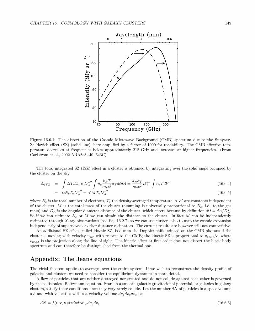
CHAPTER 16. COSMOLOGY WITH GALAXY CLUSTERS 149
Figure 16.6.1: The distortion of the Cosmic Microwave Background (CMB) spectrum due to the Sunyaev-Zel’dovich effect (SZ) (solid line), here amplified by a factor of 1000 for readability. The CMB effective tem-perature decreases at frequencies below approximately 218 GHz and increases at higher frequencies. (FromCarlstrom et al., 2002 ARA&A..40..643C)
The total integrated SZ (ISZ) effect in a cluster is obtained by integrating over the solid angle occupied bythe cluster on the sky
∆ISZ =
∫∆TdΩ ≈ D−2
A
∫nekBT
mec2σT d`dA =
kBσTmec2
D−2A
∫neTdV (16.6.4)
= αNeTeD−2A = α′MTeD
−2A (16.6.5)
where Ne is the total number of electrons, Te the density-averaged temperature, α, α′ are constants independentof the cluster, M is the total mass of the cluster (assuming is universally proportional to Ne, i.e. to the gasmass) and DA is the angular diameter distance of the cluster, which enters because by definition dΩ = dA/D2
A.So if we can estimate Ne or M we can obtain the distance to the cluster. In fact M can be independentlyestimated through X-ray observations (see Eq. 16.2.7) so we can use clusters also to map the cosmic expansionindependently of supernovae or other distance estimators. The current results are however still not competitive.
An additional SZ effect, called kinetic SZ, is due to the Doppler shift induced on the CMB photons if thecluster is moving with velocity vpec with respect to the CMB; the kinetic SZ is proportional to vpec,`/c, wherevpec,` is the projection along the line of sight. The kinetic effect at first order does not distort the black bodyspectrum and can therefore be distinguished from the thermal one.
Appendix: The Jeans equationsThe virial theorem applies to averages over the entire system. If we wish to reconstruct the density profile ofgalaxies and clusters we need to consider the equilibrium dynamics in more detail.
A flow of particles that are neither destroyed nor created and do not collide against each other is governedby the collisionless Boltzmann equation. Stars in a smooth galactic gravitational potential, or galaxies in galaxyclusters, satisfy these conditions since they very rarely collide. Let the number dN of particles in a space volumedV and with velocities within a velocity volume dvxdvydvz be
dN = f(t,x,v)dxdydzdvxdvydvz (16.6.6)
CHAPTER 16. COSMOLOGY WITH GALAXY CLUSTERS 150
where f is the distribution function and the space-velocity volume element is called the phase-space volume.Since the particle number is conserved, the number of particles with velocity vx entering in a space volumedxdydz in direction x in the time interval dt is ρdxdydx = ρvxdtdydz where ρ is the number density of particles,minus the number exiting from the other side; if the particles move only along x, this has to be equal to thechange in the number of particles inside the volume itself, dρdV . Then we have the continuity equation (theincoming velocity is taken negative)
dρdV = −d(ρvx)dtdydz (16.6.7)
or
∂ρ
∂t= −∂(ρvx)
∂x(16.6.8)
For particle moving in any direction and also with any velocity, we have the general phase-space continuityequation
∂f
∂t+
6∑i=1
∂(fwi)
∂wi= 0 (16.6.9)
where w = x, y, z, vx, vy, vz = x,v is the phase-space vector of coordinates. Now we have vi = − ∂Φ∂xi
whereΦ is the gravitational potential, and
∂wi∂wi
= ∂vi∂xi
,− ∂
∂vi
∂Φ
∂xi = 0 (16.6.10)
since the velocity vector is independent of the coordinates and the gravitational potential Φ is independent ofthe velocities. Then finally
df
dt=∂f
∂t+
6∑i=1
w∂f
∂wi= 0 (16.6.11)
or the collisionless Boltzmann equation
∂f
∂t+ v · ∇f −∇Φ · ∇f = 0 (16.6.12)
This equation can be written in any system of coordinates, eg cylindrical (useful for disk-like galaxies) orspherical (for spherical galaxies or clusters). In spherical coordinates we have
∂f
∂t+ r
∂f
∂r+ θ
∂f
∂tθ+ φ
∂f
∂φ+ vr
∂f
∂vr+ vθ
∂f
∂vθ+ vφ
∂f
∂vφ= 0 (16.6.13)
where we can also write r = vr, θ = vθ/r and φ = vφ/r sin θ (here we have defined the velocity components asthe projection of the cartesian velocity along the directions r, θ, φ, respectively).
The relation of the accelerations in terms of the potential derivatives should be derived by transforming thecorresponding cartesian expressions. Here we give directly the equations:
vr =v2θ + v2
φ
r− ∂Φ
∂r(16.6.14)
vθ =v2φ cot θ − vrvθ
r− 1
r
∂Φ
∂θ(16.6.15)
vφ =−vφvr − vφvθ cot θ
r− 1
r sin θ
∂Φ
∂φ(16.6.16)
We assume from now on that the potential is purely spherical. Then we can write
∂f
∂t+vr
∂f
∂r+vθr
∂f
∂θ+
vφr sin θ
∂f
∂φ+
(v2θ + v2
φ
r− ∂Φ
∂r
)∂f
∂vr+
(v2φ cot θ − vrvθ
r
)∂f
∂vθ+
(−vφvr − vφvθ cot θ
r
)∂f
∂vφ= 0

CHAPTER 16. COSMOLOGY WITH GALAXY CLUSTERS 151
(16.6.17)
Now we put ν(t,x) =∫fdvrdvθdvφ , which is then a density independent of velocity, and integrate the above
equation over the velocities. We have for instance terms like∫∂f
∂vrdvrdvθdvφ =
∂
∂vrν(x) = 0 (16.6.18)∫
vr∂f
∂rdvrdvθdvφ = −
∫∂vr∂r
fdvrdvθdvφ = − ∂
∂rvr (16.6.19)∫
vrvθ∂f
∂θdvrdvθdvφ = −
∫∂(vrvθ)
∂θfdvrdvθdvφ = − ∂
∂θσrθ +
∂
∂θ(vrvθ) (16.6.20)
(we applied integration by parts) where vr is the average of vr and
σ2ij =
∫vivjfdvrdvθdvφ − vivj (16.6.21)
is the velocity covariance. So we multiply by vr and obtain
vr∂f
∂t+ v2
r
∂f
∂r+vrvθr
∂f
∂θ+
vrvφr sin θ
∂f
∂φ+ vr
(v2θ + v2
φ
r− ∂Φ
∂r
)∂f
∂vr
+vr
(v2φ cot θ − vrvθ
r
)∂f
∂vθ+ vr
(−vφvr − vφvθ cot θ
r
)∂f
∂vφ= 0 (16.6.22)
We know simplify our problem by assuming that: a) the system is stationary (all time derivatives vanishand vr = 0; b) the kinematics has spherical symmetry: i.e. there is no rotation (vθ = vφ = 0) and alsoσ2rθ = σ2
rφ = σ2θφ = 0; c) finally, we also impose σ2
θθ = σ2φφ ≡ σ2
t . Then we have the Jeans equation
1
ν
∂
∂r(νσ2
rr) + 2σ2rr − σ2
t
r= −∂Φ
∂r= −GM(r)
r2(16.6.23)
or
1
ν
∂
∂r(νσ2
rr) + 2σ2rr
β
r= −∂Φ
∂r= −GM(r)
r2(16.6.24)
where
β = 1− σ2t
σ2rr
(16.6.25)
is the anisotropy parameter, and it can take values in −∞ < β ≤ 1. Notice that here the mass M includesall sources of gravity while the density ν might refer only to a particular population, eg stars or galaxies, andnot necessarily to all the matter in the system. If velocities are isotropic, σ2
rr = σ2t we obtain the condition of
spherical hydrostatic equilibrium
1
ν
∂
∂r(νσ2
rr) = −GM(r)
r2(16.6.26)
The Jeans equation can be written in a form that directly gives the mass profile as a function of observables
M(r) = −rσ2rr
G
[d lnν
d lnr+d lnσ2
rr
d lnr+ 2β(r)
](16.6.27)
Notice the similarity to the hydrostatic equation (16.2.4). However, the function β(r) is very difficult to estimate,since we only directly measure the line-of-sight velocity.
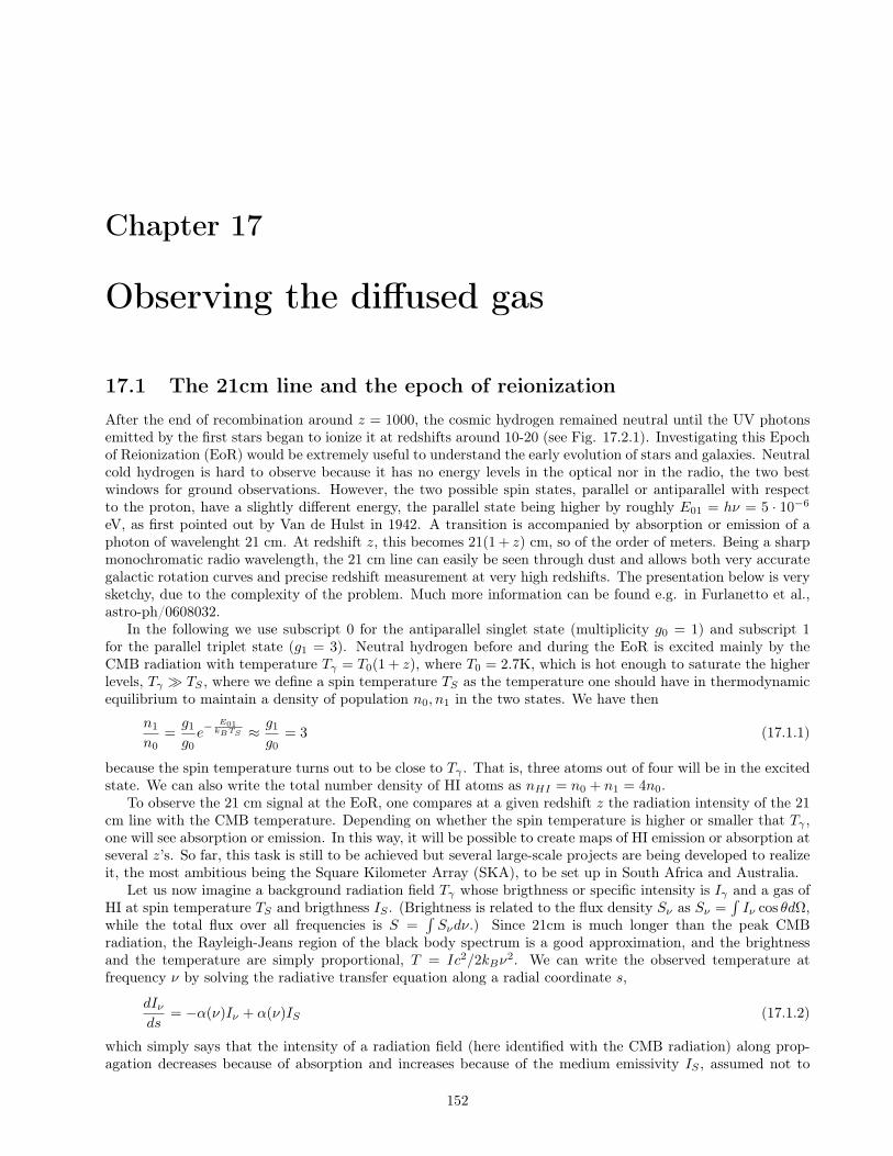
Chapter 17
Observing the diffused gas
17.1 The 21cm line and the epoch of reionizationAfter the end of recombination around z = 1000, the cosmic hydrogen remained neutral until the UV photonsemitted by the first stars began to ionize it at redshifts around 10-20 (see Fig. 17.2.1). Investigating this Epochof Reionization (EoR) would be extremely useful to understand the early evolution of stars and galaxies. Neutralcold hydrogen is hard to observe because it has no energy levels in the optical nor in the radio, the two bestwindows for ground observations. However, the two possible spin states, parallel or antiparallel with respectto the proton, have a slightly different energy, the parallel state being higher by roughly E01 = hν = 5 · 10−6
eV, as first pointed out by Van de Hulst in 1942. A transition is accompanied by absorption or emission of aphoton of wavelenght 21 cm. At redshift z, this becomes 21(1 + z) cm, so of the order of meters. Being a sharpmonochromatic radio wavelength, the 21 cm line can easily be seen through dust and allows both very accurategalactic rotation curves and precise redshift measurement at very high redshifts. The presentation below is verysketchy, due to the complexity of the problem. Much more information can be found e.g. in Furlanetto et al.,astro-ph/0608032.
In the following we use subscript 0 for the antiparallel singlet state (multiplicity g0 = 1) and subscript 1for the parallel triplet state (g1 = 3). Neutral hydrogen before and during the EoR is excited mainly by theCMB radiation with temperature Tγ = T0(1 + z), where T0 = 2.7K, which is hot enough to saturate the higherlevels, Tγ TS , where we define a spin temperature TS as the temperature one should have in thermodynamicequilibrium to maintain a density of population n0, n1 in the two states. We have then
n1
n0=g1
g0e− E01kBTS ≈ g1
g0= 3 (17.1.1)
because the spin temperature turns out to be close to Tγ . That is, three atoms out of four will be in the excitedstate. We can also write the total number density of HI atoms as nHI = n0 + n1 = 4n0.
To observe the 21 cm signal at the EoR, one compares at a given redshift z the radiation intensity of the 21cm line with the CMB temperature. Depending on whether the spin temperature is higher or smaller that Tγ ,one will see absorption or emission. In this way, it will be possible to create maps of HI emission or absorption atseveral z’s. So far, this task is still to be achieved but several large-scale projects are being developed to realizeit, the most ambitious being the Square Kilometer Array (SKA), to be set up in South Africa and Australia.
Let us now imagine a background radiation field Tγ whose brigthness or specific intensity is Iγ and a gas ofHI at spin temperature TS and brigthness IS . (Brightness is related to the flux density Sν as Sν =
∫Iν cos θdΩ,
while the total flux over all frequencies is S =∫Sνdν.) Since 21cm is much longer than the peak CMB
radiation, the Rayleigh-Jeans region of the black body spectrum is a good approximation, and the brightnessand the temperature are simply proportional, T = Ic2/2kBν
2. We can write the observed temperature atfrequency ν by solving the radiative transfer equation along a radial coordinate s,
dIνds
= −α(ν)Iν + α(ν)IS (17.1.2)
which simply says that the intensity of a radiation field (here identified with the CMB radiation) along prop-agation decreases because of absorption and increases because of the medium emissivity IS , assumed not to
152

CHAPTER 17. OBSERVING THE DIFFUSED GAS 153
Figure 17.1.1: Absorption of a Lyman-α line (adapted from Wikicommons, authors OrangeDog and Szdori,license CC-BY-2.5).
depend on s. We define the optical depth
τ =
∫α(ν)ds (17.1.3)
where α(ν) is the absorption coefficient at frequency ν and ds integrates along the line of sight. (Note that allfrequencies in what follows are rest frame values, not redshifted ones.) The solution for the observable brightnessIB is
IB = IS(1− e−τ ) + Iγe−τ (17.1.4)
Since in the Rayleigh-Jeans regime T is proportional to I, we can also write
TB = TS(1− e−τ ) + Tγe−τ (17.1.5)
where also TB scales with redshift as (1 + z). As intuitive, if the material is optically thick, τ 1, we see thespin temperature, if optically thin, τ 1, we see the CMB background. This relation can also be written as
TB0(1 + z) = TS(1− e−τ ) + T0(1 + z)e−τ (17.1.6)
and therefore
δTB ≡ TB0 − T0 =TS − Tγ
1 + z(1− e−τ ) (17.1.7)
The quantity δTB , called brigthness, is the main observable: the difference between the observed and the CMBtemperature at the desired frequency. Now we need to estimate τ and TS .
The absorption coefficient gives the loss of energy per unit frequency of a radiation field resulting fromabsorption of photons (0→ 1) minus stimulated emission (1→ 0). Since τ is dimensionless, α(ν) has dimensionsm−1. We need to introduce then the Einstein coefficients Bab for the transition a→ b : the Einstein coefficient isthe probability per unit time per unit spectral energy density, where the spectral energy is the energy density perunit frequency, so Bab has units J−1m3s−2. The rate (i.e. the probability per unit time) of absorption/emissionis then given by Babhνnφ(ν), where n is the number density of absorbers (atoms), φ(ν) the line profile normalized
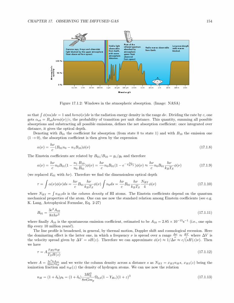
CHAPTER 17. OBSERVING THE DIFFUSED GAS 154
Figure 17.1.2: Windows in the atmospheric absorption. (Image: NASA)
so that∫φ(nu)dν = 1 and hνnφ(ν)dν is the radiation energy density in the range dν. Dividing the rate by c, one
gets αab = Babhνnφ(ν)/c, the probability of transition per unit distance. This quantity, summing all possibleabsorptions and substracting all possible emissions, defines the net absorption coefficient: once integrated overdistance, it gives the optical depth.
Denoting with B01 the coefficient for absorption (from state 0 to state 1) and with B10 the emission one(1→ 0), the absorption coefficient is then given by the expression
α(ν) =hν
c(B01n0 − n1B10)φ(ν) (17.1.8)
The Einstein coefficients are related by B01/B10 = g1/g0 and therefore
α(ν) =hν
cn0B01(1− n1
n0
B10
B01)φ(ν) =
hν
cn0B01(1− e−
hνkBTS )φ(ν) ≈ hν
cn0B01
hν
kBTSφ(ν) (17.1.9)
(we replaced E01 with hν). Therefore we find the dimensionless optical depth
τ =
∫α(ν)φ(ν)ds =
hν
cB01
hν
kBTSφ(ν)
∫n0ds =
hν
cB01
hν
kBTS
NHI4
φ(ν) (17.1.10)
where NHI =∫nHIds is the column density of HI atoms. The Einstein coefficients depend on the quantum
mechanical properties of the atom. One can use now the standard relation among Einstein coefficients (see e.g.K. Lang, Astrophysical Formulae, Eq. 2-27)
B01 =3c3A10
8πhν3(17.1.11)
where finally A10 is the spontaneous emission coefficient, estimated to be A10 = 2.85× 10⁻¹⁵s−1 (i.e., one spinflip every 10 million years!).
The line profile is broadened, in general, by thermal motion, Doppler shift and cosmological recession. Herethe dominating effect is the latter one, in which a frequency ν is spread over a range ∆ν
ν ≈∆Vc where ∆V is
the velocity spread given by ∆V = sH(z). Therefore we can approximate φ(ν) ≈ 1/∆ν ≈ c/(sH(z)ν). Thenwe have
τ = AxHInHTSH(z)
(17.1.12)
where A = 3c3hA10
32πν2kBand we write the column density across a distance s as NHI = xHInHs, xHI(z) being the
ionization fraction and nH(z) the density of hydrogen atoms. We can use now the relation
nH = (1 + δb)ρb = (1 + δb)3H2
0
8πGmpΩb,0(1− YHe)(1 + z)3 (17.1.13)

CHAPTER 17. OBSERVING THE DIFFUSED GAS 155
(the factor of mp, mass of the proton, is needed to convert the energy density ρb into the number density nH)where δb is the fluctuation in the baryon content and YHe ≈ 0.245 is the fraction in mass in Helium (all therest being hydrogen). We use also H(z) = H0Ω
1/2m,0(1 + z)3/2, and finally we obtain from (17.1.7) and τ 1 the
brigthness
δTB ≈TS − Tγ
1 + zτ =
3
8πGmpA(1− Tγ
TS)xHI(1 + δb)Ωb,0(1− YHe)H2
0 (1 + z)2
TSH(z)(17.1.14)
=3H0A(1− YHe)
8πGmp(1− Tγ
TS)xHI(1 + z)1/2 Ωb,0
Ω1/2m,0
(17.1.15)
≈ 27xHI(1 + δb)(1−TγTS
)(1 + z
10
0.15
Ωm,0h2)1/2(
Ωb,0h2
0.023)mK (17.1.16)
where the last expression allows an immediate estimation of the order of magnitude, since all factors are of orderunity. This expression can be further corrected by multiplying it by H/(dv/dr + H), where dv/dr gives thecontribution to the line width due to the peculiar velocities along the line of sight. If TS > Tγ , the brigthnessδTB is positive (emission). Detection of δTB can therefore map the history of reionization xHI(z), measure acombination of Ωb and Ωm, and map the spatial and time structure of the fluctuations in the baryon componentδb.
To estimate TS we should take into account three processes: 1) absorption and stimulated emission of CMBphotons; 2) collisions with other hydrogen atoms, free electrons, and protons; and 3) Lyman-α photons (UV)scattering. We denote with C10, P10 the de-excitation rates per atom from collisions and UV scattering, andwith C01, P01 the corresponding excitation rates. At equilibrium we have then
n1(C10 + P10 +A10 +B10Iγ) = n0(C01 + P01 +A01 +B01Iγ) (17.1.17)
Now we can replace Iγ with Tγ using the Rayleigh-Jeans relation. Then we can invoke detailed equilibrium andwrite
C01
C10=g1
g0e− hvkBTK ≈ 3(1− hν
kBTK) (17.1.18)
where TK is the kinetic temperature, and similarly define an effective “color temperature” of the UV ionizingfield Tc via
P01
P10≡ 3(1− hν
kBTc) (17.1.19)
Putting all this into (17.1.17) we find
T−1S =
T−1γ + xcT
−1K + xαT
−1c
1 + xc + xα(17.1.20)
where
xc =C10
A10
hν
kBTγ(17.1.21)
xα =P10
A10
hν
kBTγ(17.1.22)
are the coupling coefficients for collisions and scattering, respectively. In the limit in which the couplings aresmall, TS = Tγ as one should expect. In most cases we can assume Tc ≈ Tγ . The exact estimation of TS can beachieved only numerically. Depending on which process dominates, one can have TS larger or small than Tγ .During the most interesting phase of reionization, at redshifts around 10, one has positive brightness, as can beseen from Fig. (17.1.3).

CHAPTER 17. OBSERVING THE DIFFUSED GAS 156
Figure 17.1.3: 21cm signal from ionized hydrogen (from Pritchard and Loeb, 2010, Nature 468, 772, reproducedwith permission).
Figure 17.2.1: Reionization history (fraction of free electrons ≈ fraction of ionized hydrogen atoms). Imagefrom Glover et al., Atomic, Molecular, Optical Physics in the Early Universe, 2014, adapted from Sunyaev andChluba (RMA, 2009).

CHAPTER 17. OBSERVING THE DIFFUSED GAS 157
17.2 Lyman-α forest
The EoR ends around z ≈ 6 but pockets of neutral hydrogen remain inside or nearby structures, e.g. alongfilaments, protected by the UV photons by their own high density. Since these clouds are associated with largescale structure, they can constitute a valuable way to reconstruct matter fluctuations at high redshifts. Theclouds can be seen as Lyman-αabsorbers (transition from n = 2 to n = 1 orbitals) along the line of sight ofdistant quasars, as in Fig. (12.7.1). Since the Lyman-α occurs at a rest frame wavelength of 1215 angstroms(≈100 nm), it falls in the UV region. When rdshifted by a factor of 1 + z equal to 3 to 6, therefore, falls in thevisible part and can be detected from the ground. Distant quasars at redshifts larger than 3 show hundreds ofthese lines, each one generated by absorption of different clouds distributed with different redshifts along theline of sight. After z ≈ 6, the end of the EoR, the lines merge into a continuous trough, called Gunn-Petersontrough: at earlier epochs the medium becomes more and more neutral.
Lyman alpha forest systems have a density of 1014 atoms per square centimeter. The so-called Lyman limitsystems are 103 times denser, while damped Lyman alpha systems another factor of 103 more. Some recentsurveys like the 2dF-SDSS quasar survey (2SLAQ) colected 100k quasars as of 2010, while BOSS DR9 cobtains180k quasars, 62k at redshifts >2.2. This high statistics allows the estimation of the 3D matter power spectrumfrom the 1D lines of sight: this is particularly useful both because the Lyman−α lines probe an epoch which isout of reach for today’s redshift surveys and because at that epoch the fluctuations are linear down to a muchsmaller scale than today’s structure (fluctiations at redshift z are roughly (1 + z) times weaker than today).The power spectrum reconstruction however requires the use of N-body simulations to understand how well theLyman−α forest traces the matter fluctuations. In Fig. (12.1.1) one can see how the Lyman−α reconstructionextends the reach of the power spectrum to small scales.

Chapter 18
Dark matter
We have mentioned several times the dark matter and have seen some of the evidence in favor of it. This chapteris devoted to the main observational techniques to “observe” dark matter beyond those already mentioned andto a short review of the candidates.
Quick summary• Dark matter is very likely non-baryonic and composed of free particles.
• Several particle physics models of DM have been proposed but the so-called WIMPs (predicted in super-symmetry) are probably the most widely accepted candidate
• WIMPs of mass 10-100 GeV would have the right amount of density to explain all of the DM
• DM can be detected directly or indirectly, or even produced in accelerators, but so far no conclusiveevidence has been reported
• Direct detection might occur when the galaxy halo DM particles cross the Earth and hit a nucleus in theunderground detectors
• Indirect detection occurs if DM annihilates when encountering other DM particles in high-density regions(central Milky Way, dwarf galaxies, clusters etc) or decays: we can then observe the products as highenergy monochromatic photons, neutrinos, charged leptons.
• Current cold DM models cannot explain easily the galaxy inner profiles and the number of dwarf satellites:this could be a problem related to baryonic physics or require a modification of the standard DM models.
18.1 Dark matter candidatesDark matter can be composed in principle by any sort of matter that escapes direct observation in everyelectromagnetic waveband, from γ-rays to radio. However we know from big bang nucleosynthesis and CMBconstraints that the baryons can only amount to 5% at most of the cosmic density, while we need around 30%of matter to explain spiral rotation curves, X−ray ICM, CMB, cosmic expansion etc. This DM must be coldenough to remain within galaxy and cluster halos: relativistic particles would easily escape the gravitationalpotentials. Moreover, the DM particles obviously have to have a mass sufficient to provide the required density.So the natural candidates are massive, cold, stable particles that do not interact electromagnetically. Sincethe existence of an abundant number of micro black holes and in general of unseen compact objects is severelylimited by many constraints (for instance, limits coming from microlensing), it is likely that the DM is a gas ofsuch particles freely floating around in galaxies and clusters.
DM particles that feel weak interaction (beside of course gravitational interaction) are called WIMPs (weaklyinteracting massive particles). In this case, one can estimate their present number density since we know theepoch when weak interacting particles left thermal equilibrium with the other particles (freezing) in the early
158
CHAPTER 18. DARK MATTER 159
Figure 18.1.1: Matter power spectrum in models with massless and massive neutrinos (from Wong, Y., Ann.Rev.Nucl.Part.Sci. 61, 2011). The data points are from the 2dF survey (Cole et al. 2005).
universe. It turns out that particles with weak-scale mass around 100 GeV will have automatically more or lessthe density required to provide all the DM we need: this is called the WIMP miracle. This feature makes theWIMPs the perfect candidate for DM. However, so far no WIMP has ever been captured or produced.
Supersymmetric theories provide a host of new partner particles to the standard model, all with masses aboveseveral GeV (otherwise they would have been produced in accelerators; this does not apply to the gravitinohowever). The lightest supersymmetric particle must be stable because there are no symmetry-conservingparticles they can decade to, so supersymmetry provide naturally at least one kind of WIMP, often identifiedwith the neutralino o gravitino or, generically, LSP, “lightest sypersymmetric particle”, whichever it be. Mostexperiments are therefore geared at capturing 10-100 GeV WIMPs passing through the Earth. The fact thatthe LHC is not finding new physics at these mass scales is generating tension with the WIMP-DM connectionscenario.
Another dark matter candidate is the axion, a particle proposed in order to understand why QCD does notviolate parity to a higher degree. Its mass is constrained to be very small, of the order of µeV, but it is stillof the “cold” type because it has never been in thermal equilibrium with the other particles. Searches for theaxion have been unsuccessful so far and large chunks of the interesting parameter space have been excluded.
Many other types of DM have been proposed, also of the “warm” type, for instance sterile neutrinos withmass around keV. One type of DM is certainly realized in nature: neutrinos. Since their mass is constrainedto be below roughly 1eV, they are born relativistic (temperature of freezing in the early universe much higherthan their mass) and might be becoming non-relativistic just now. Such a small mass implies that they cannotcontribute to a large fraction of the DM, at most 1%. Moreover, their large velocity will not allow them tocluster along with baryonic matter so that they will in general decrease the overall matter clustering. In fact,by measuring accurately the matter power spectrum one can infer upper limits to the abundance, and thereforemass, of the neutrinos. In agreement with neutrino oscillation experiments, cosmology constrains the neutrinomass to be at or below the eV level (see Fig. 18.1.1).
18.2 Direct detectionIf dark matter forms a giant halo around the bulge and disk of the Milky Way then the DM particles shouldcross the Earth and can be in principle detected through their weak interaction with nuclei. The density of thehalo should be roughly 100 times the background density, i.e. around 0.3 proton mass per cm3 so if the DMparticles have a mass of say 100 GeV there should be one DM particle every liter of space. If the DM halo isslowly rotating, the Earth will feel a wind of DM particles at a velocity of 220 km/sec (the velocity of the Sunaround the Milky Way center), with a little annual modulation along the Earth’ orbit around the Sun, for a

CHAPTER 18. DARK MATTER 160
Figure 18.2.1: Typical exclusion plot cross section versus DM mass collecting the results of many exper-iments (XENON collaboration, 2012). The closed contours (DAMA, CoGent, CRESST) are positive de-tections, which appear therefore in contrast with the excluded regions from other experiments. (Credits:http://xenon.astro.columbia.edu/XENON100_Experiment/ and Phys. Rev. Lett. 109, 181301 (2012))
total rate of 104÷5 particles per square centimeter per second.Some of these non-relativistic particles will hit, although with a very low probability, the nuclei of the
detectors currently located in various underground laboratories, shielded from the cosmic ray noise by kilometersof rock. A typical event rate could be up to a few events per day per kilogram of detector. Since we expecta good mass range to be around 10-100 GeV, the DM detectors normally employ nuclei with similar mass likeGermanium, Silicon, Iodium in order to maximize the recoil. The energy of the recoil is in any case extremelysmall, up to 100 keV. The recoil can then be measured because, depending on the detector substance, it createscrystal dislocations, ionization, phonons, scintillations.
The main problem is separating true DM events from background, mostly due to natural radioactivity ofthe rocks and of the detector material itself. Another way is to search for the small annual modulation due tothe Earth orbit: the experiment DAMA at Gran Sasso, Italy, claims since several years a positive detection butso far it has not received robust confirmation. Most experiments produced regions of excluded parameter spacein the plane cross section versus mass (Fig. 18.2.1). Low cross sections and low masses are clearly more difficultto constrain and ample regions of parameter space are still unconstrained.
Another form of “almost direct” detection is DM production at high-energy accelerator like LHC at CERN.If the collision of two protons or other particles generates products that do not add up to the original energy,it means some particles have escaped detection. A careful series of tests on backgrounds and on already knownelusive particles might in principle lead to the conclusion that the escaped particles are DM candidates.
18.3 Indirect detectionDM particles can be indirectly detected if we can observe signals that are linked to DM decay or self-annihilation.One possibility is that after many interactions some DM particles lose energy and are eventually gravitationallycaptured by the Sun (or even the Earth). If they accumulate for billion years in the core of the Sun theirdensity might become large enough that their annihilation rate becomes significant. Neutrinos generated bythe annihilation will be much more energetic than thermonuclear solar neutrinos and will impact the Earthatmosphere and rock, creating muons. If in a underground laboratory a highly energetic muon traveling upwardis observed, it cannot come from cosmic rays hitting the atmosphere, so one possibility is that it comes fromneutrinos generated in the Earth or Sun’s core by DM annihilation. The high-energy neutrinos can also be

CHAPTER 18. DARK MATTER 161
Figure 18.3.1: Excess of antiproton/proton ratio from the experiments PAMELA and AMS-02. The data arejust above the uncertainty band (from Giesen et al. 2015, Journal of Cosmology and Astroparticle Physics,Issue 09, article id. 023, (2015)).
directly captured by neutrino detectors like AMANDA and IceCube.Another signal from annihilating or decaying DM can be obtained looking for 100 GeV-range γ-ray photons
from space, perhaps from regions where we expect a high angular concentration of DM, for instance in thedirection of M31 (Andromeda galaxy), the Large Magellanic Cloud, dwarf galaxies in the Local Group, theMilky Way center, galaxy clusters. Since the annihilation is a two-particle process, it is proportional to the DMdensity squared and this might help revealing the effect and distinguishing it from astrophysical backgrounds(for instance pulsars and supernovae remnants). The photons should have exactly the energy of the DM particlesand therefore appear as a sharp line on the continuum coming from high-density regions (redshifted if comingfrom a moving source). Notwithstanding various temptative detections, so far the satellite Fermi-LAT hasexcluded WIMP masses up to 100 GeV. Cherenkov detectors, like HESS, MAGIC, VERITAS on Earth can alsocollect the particle showers generated from the impact of the high-energy photons with the atmosphere.
DM annihilation/decay products could also be pairs of charged fermions (protons, electrons and their antipar-ticles). The antiparticles will generate an excess over the standard astrophysical background particle/antiparticleratio and could be revealed by the satellite PAMELA and the instrument AMS on board the ISS. Here againseveral detection claims have arisen but none has proven to be conclusive evidence of new physics (see Fig.18.3.1).
18.4 The problems of the cold dark matterAlthough the CDM is widely regarded as the most likely form of dark matter, it is not without problems.The main problem is the excess of small substructure we see (and expect to see) in N -body simulations withrespect to what we observe in galaxies (Fig. 18.4.1). The high-mass end disagreement is not so critical becauselarge halos will in general host groups or clusters instead of individual galaxies. Since CDM does not dissipateefficiently because weakly interacting, and because the theoretical power spectrum has no natural cut-off scale,the CDM lumps formed under gravitational instability live practically forever as satellites within the halos oflarge galaxies as ours. But around the Milky Way we observe only a few dozen dwarf galaxies, although wecannot easily estimate how many (perhaps hundreds) we are missing due to low surface brightness. Of course wedo not know whether every DM lump should contain stars or instead just remain dark either because not enoughbaryons are collected or because they remain too hot to collapse into stars. So in fact the DM subclusteringproblems is probably just a manifestation of our uncertainties about baryonic physics, that is, of exactly how

CHAPTER 18. DARK MATTER 162
Figure 18.4.1: Halo mass function from N -body simulations (dahed lines) compared with the galaxymass/luminosity function from real data (continuous and dotted lines). The discrepancy means that thereis a non-linear relation between halos and galaxies. In particular, at the small mass end, the simulations showmuch more halos than galaxies (from Baldry et al., On the galaxy stellar mass function, the mass–metallicityrelation and the implied baryonic mass function, Mon. Not. R. Astron. Soc. 388, 945–959 (2008)).
and when exactly stars finally form.The clustering problem of DM arises at small scales and its consequence is not just an excess of satellites
but also a inner halo profile that seem much steeper (cuspy) that the one that best fits galaxy rotation curves:this is called the cusp-core problem. Here again the DM evidence comes from N -body simulations, well fittedby the steep NFW profile (12.7.2), while observations refer to luminous sources, so baryonic physics might verylikely play an important role. Alternatively, DM could depart from the simplest theoretical expectations andallow for a stronger self-interaction that introduces some form of dissipative friction that erases substructure.

Appendix
163
Probability distributions
Some well-known probability distributions.Poisson distribution.The Poisson distribution gives the probability to have N events when η are expected. For instance, if
we throw at random balls in a set of boxes, so that the boxes contain on average η balls each, the Poissondistribution gives us the probability to find N balls in a given box. It is given by the PDF
P (N ; η) =e−ηηN
N !(18.4.1)
Although the Poisson distribution is defined over integer numbers, we can approximate it as a continuousdistribution for large η. The PDF is normalized to unity, and its average is of course η, while its variance isalso η. For instance, if the average number of balls is 3, there is a 5% chance to get no balls in a given box.This gives a simple prescription for the variance to be expected in a distribution of particles, eg galaxies, whenthe process that created the distribution is supposed to be uniform: if we find N galaxies in a given volume,then we can estimate the variance as N , and therefore the error on N will be
√N. This is the often employed
Poissonian error.Gaussian distributionThe Gaussian distribution is
P (x) = (2πσ2)−1/2 exp
[− (x− x0)2
2σ2
](18.4.2)
Its mean is x0 and its variance is σ. The Gaussian distribution describes the distribution of a random variablewhen the variable is the result of many independent processes; for instance, a measure is subject to manyexperimental uncertainties, most of which are independent, and so the measure itself can be approximatelydistributed as a gaussian around its true value.
χ2 distributionThe χ2 distribution is
P (χ2;n) =(χ2)n/2−1 exp(−χ2/2)
2n/2Γ(n/2)(18.4.3)
Its mean is n and its variance is 2n. The χ2 distribution is useful because a sum of n squared Gaussian variablesis distributed as a χ2 variable. Since a product of Gaussian distribution can be expressed as a function of thesum of squared Gaussian variables, the χ2 PDF gives the resulting distribution.
164


