Lecture Notes: Estimation of dynamic discrete choice models∗

Jean-Francois HoudeCornell University

November 7, 2016

∗These lectures notes incorporate material from Victor Agguirregabiria’s graduate IO slides at the University of Toronto(http : //individual.utoronto.ca/vaguirre/courses/eco2901/teaching io toronto.html).

1

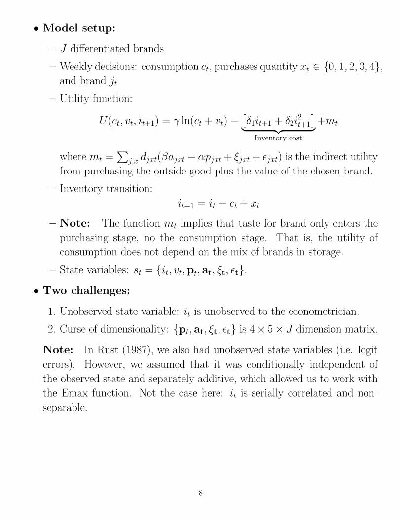
Demand for storable goods

• Key references:

– Pesendorfer (2002)

– Erdem, Imai, and Keane (2003)

– Hendel and Nevo (2006a) and Hendel and Nevo (2006b)

• If consumers can stockpile a storable good, they can benefit from “sales”:

purchase more than consumption when prices are low.

• This creates a difference between purchasing and consumption elasticity

– In the short-run, store-level demand elasticity reflect stockpiling behav-

ior

– In the long-run, store-level demand elasticity reflects consumption de-

cisions

• Ignoring stockpiling and forward-looking behavior can lead to biases: own

and cross price elasticities.

• If consumers differ in the storage costs firms have an incentive to price

discriminate: PD theory of sales.

• Ketchup pricing example (Pesendorfer 2002):

2

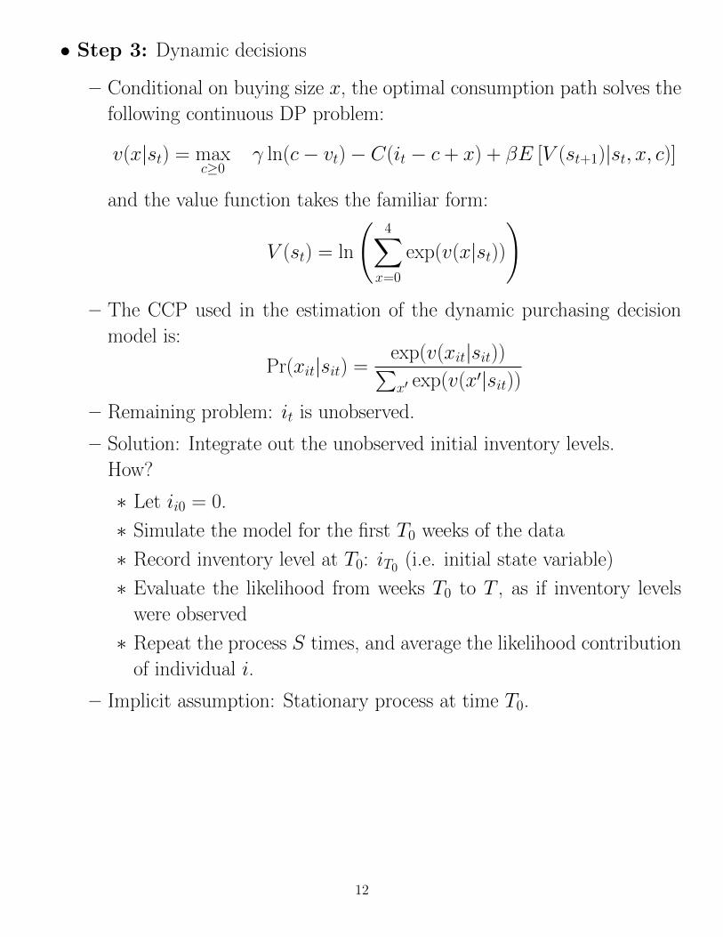
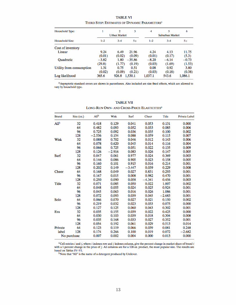
• Hendel and Nevo (2006a):

– Estimate an inventory control model with product differentiation

– Two challenges: (i) inventories are unobserved (key state variable), and

(ii) differentiation creates a dimensionality problem

– Propose a simplifying assumption that: (i) reduce the computation

burden of the model (reduce the dimension), and (ii) simplify the esti-

mation (three-step algorithm).

• Data:

– Scanner data: Household panel with purchasing decisions from 1991-

1993

– Firms: 9 supermarkets (ignore supermarket choice)

– Store-level data: choice-set and product attributes (detergent), promo-

tions, and prices

3

• Market shares and sales:

4

• Descriptive evidence (Hendel and Nevo 2006b)

– Issue: Inventories are unobserved

– Duration since previous sale promotion is positively correlated with

aggregate quantity purchased

– Proxy for inventory cost (e.g. house size, dog) are negatively correlated

with propensity to buy on sale

5

6

7

• Model setup:

– J differentiated brands

– Weekly decisions: consumption ct, purchases quantity xt ∈ 0, 1, 2, 3, 4,and brand jt

– Utility function:

U(ct, vt, it+1) = γ ln(ct + vt)−[δ1it+1 + δ2i

2t+1

]︸ ︷︷ ︸Inventory cost

+mt

where mt =∑

j,x djxt(βajxt− αpjxt + ξjxt + εjxt) is the indirect utility

from purchasing the outside good plus the value of the chosen brand.

– Inventory transition:

it+1 = it − ct + xt

– Note: The function mt implies that taste for brand only enters the

purchasing stage, no the consumption stage. That is, the utility of

consumption does not depend on the mix of brands in storage.

– State variables: st = it, vt,pt, at, ξt, εt.

• Two challenges:

1. Unobserved state variable: it is unobserved to the econometrician.

2. Curse of dimensionality: pt, at, ξt, εt is 4× 5× J dimension matrix.

Note: In Rust (1987), we also had unobserved state variables (i.e. logit

errors). However, we assumed that it was conditionally independent of

the observed state and separately additive, which allowed us to work with

the Emax function. Not the case here: it is serially correlated and non-

separable.

8

• Model choice-probability:

Pr(djxt = 1|st) =exp (βajxt − αpjxt + ξjxt +M(x, st))∑

x′,j′ exp (βaj′x′t − αpj′x′t + ξj′x′t +M(x′, st))

Where,

M(x, st) = maxcγ ln(c+ vt)−

[δ1it+1 + δ2i

2t+1

]+ βE [V (st+1)|x, c, st]

s.t. it+1 = it − c+ x

• Note that conditional on purchasing size x, the brand choice is a staticproblem:

Pr(djt = 1|st, xt = x) =exp (βajxt − αpjxt + ξjxt +M(x, st))∑j′ exp (βaj′xt − αpj′xt + ξj′xt +M(x, st))

=exp (βajxt − αpjxt + ξjxt)∑j′ exp (βaj′xt − αpj′xt + ξj′xt)

This probability can be estimated by MLE: Multinomial logit model.

• This is the first-step of the estimation procedure.

• Endogenous prices and advertising? Brand/size fixed-effects, such that

ξjxt = ξjx.

9

• How to deal with the dimensionality problem?

• Since the brand-choice is static, we can write down the expected utility (i.e.

Emax) conditional on size:

ωt(x) = E

(maxjβajxt − αpjxt + ξjxt + εjt

)= ln

J∑j=1

exp (βajxt − αpjxt + ξjxt)

• McFadden (1978) calls ωt(x) the “inclusive values”. It summarizes the

information contained in the vector of prices and characteristics available

in period t, very much like a quality-adjusted price index.

• Dynamic programming problem re-defined:

V (it, vt, ωt, εt) = maxc,x

γ ln(c− vt)− C(it+1) + ωt(x) + εxt

+βE [V (it+1, vt+1, ωt+1, εt+1)|it, vt, ωt, εt, x, c)]

• To be able to define the state-vector solely as (it, vt, ωt, εt), we need to

impose an addition assumption on the transition process of ωt:

Pr(ωt+1|at, pt, ξt) = Pr(ωt+1|ωt)

This assumption as been called the “Inclusive-value sufficiency” assumption

(Gowrisankaran and Rysman 2012).

10

• Step 2: Estimate the Markov process for ωt(x)

11

• Step 3: Dynamic decisions

– Conditional on buying size x, the optimal consumption path solves the

following continuous DP problem:

v(x|st) = maxc≥0

γ ln(c− vt)− C(it − c + x) + βE [V (st+1)|st, x, c)]

and the value function takes the familiar form:

V (st) = ln

(4∑

x=0

exp(v(x|st))

)– The CCP used in the estimation of the dynamic purchasing decision

model is:

Pr(xit|sit) =exp(v(xit|sit))∑x′ exp(v(x′|sit))

– Remaining problem: it is unobserved.

– Solution: Integrate out the unobserved initial inventory levels.

How?

∗ Let ii0 = 0.

∗ Simulate the model for the first T0 weeks of the data

∗ Record inventory level at T0: iT0 (i.e. initial state variable)

∗ Evaluate the likelihood from weeks T0 to T , as if inventory levels

were observed

∗ Repeat the process S times, and average the likelihood contribution

of individual i.

– Implicit assumption: Stationary process at time T0.

12

13

• Two differences between static and dynamic model:

1. Static model implies larger price coefficient,

2. and ignores the inventory problem

• Both lead to a larger own price elasticity with the static model, than the

long-run own price elasticity with the dynamic model.

• Point two leads to a lower cross price elasticity (with the static model).

Why?

– In the data the response to sales is mostly coming from people going

from not buying to buying the brand on sale.

– This leads to predict small cross price elasticities with respect to other

products, and large cross price elasticity with respect to the outside

good.

– Or more mechanically, in the static model, the choice probability are all

relatively small since consumers buy detergent infrequently. The logic

cross-partials are equal to the product of the two choice-probabilities:

small cross-elasticities.

– The dynamic model rationalize this phenomenon high unobserved in-

ventories, and conditional choice probabilities (conditional on purchas-

ing). Everybody needs detergent...

14

Demand for durable goods

Motivation:

• In many settings, the timing of purchase is as important as what you

purchase.

• In durable goods markets, this is true because the quality and price of

products available at any point in time vary less, than the quality and

price of products offer across time.

• Why? Introduction of new products push the technology frontier upwards,

and most firms often respond by using dynamic pricing strategy (i.e. dis-

count products that are about to be discontinued).

• Challenges: (i) Micro data on product replacement is rare, and (ii) dynamic

“engine” replacement models with product differentiation have very large

state space.

• Examples: Gordon (2010), Gowrisankaran and Rysman (2012)

15

Model: Gowrisankaran and Rysman (2012)

• Indirect utility over product characteristics (omit time):

Uij = βixj + ξj + εij = δj + µij + εij = uij + εij (1)

• Utility over current product:

Ui0 = βix0 + εi0 = ui0 + εi0 (2)

Note: product 0 is either the outside option (not using a camcorder), or

the last camcorder purchased. GR assume that products do not depreciate,

and there are no sunk replacement costs.

• Bellman equation:

– Multinomial choice: ai ∈ Ai = 0, 1, ..., J. Where J is the current

number of products available.

– Common state-space: si = ui0, x1, ..., xJ , p1, ..., pJ– Expected Bellman equation:

Vi(si) = Eε

[maxa∈Ai

ui,a − αipia + εia + βEs′(Vi(s

′)|si, a))]

= Eε

[max

vi(0|si) + εi0, max

a∈A\0vi(a|si) + εia

]where pia = 0 if a = 0, and vi(a|si) = uia−αipia+βEs′

(Vi(s

′)|si, a)).

• Curse of dimensionality: (i) The number of grid points to approxi-

mate Vi(si) grows exponentially with the number of products, and (ii) The

calculation of the continuation value involves a |s| dimension integral (i.e.

Es′(V |x)).

16

Dimension reduction assumption:

• Recall that if εij is distributed according to a type-1 extreme value distri-

bution with location/spread parameters (0, 1), then maxa∈A\0 vi(a|x) + εiais also EV1 distributed with location parameter:

ωi(si) = log

∑a∈A\0

exp(vi(a|si))

and spread parameter of 1.

• ωi(si) is the expected discounted value of buying the preferred camcorder

available today, instead of holding to the current one (i.e. outside option).

• Therefore, we can rewrite the expected Bellman equation as:

Vi(si) = Eε [max vi(0|si) + εi0, ωi(si) + εi1]= log (exp(vi(0|si)) + exp(ωi(si)))

• So far, we’re simply re-writing the problem so that it looks more like a

sequential decision problem: (i) replace or not replace, and (ii) which new

product to buy conditional on replacing. The value of replacing is ωi(si).

• In order to reduce the dimension of the state space, GR introduce a new

assumption:

Inclusive value sufficiency: If ωi(si) = ωi(si), then gω (ωi(s′)|si) =

gω (ωi(s′)|si)). Where gω(x|si) is the density of the option value ω.

• Importantly, this implies that if two different states have the same option

value ω, then they also have the same value function.

• In addition, we assume that ωi evolves over time according to an AR(1)

process:

ωi,t+1 = ρi,0 + ρi,1ωi,t + ηi,t+1

where ηi,t is mean zero shock.

17

• The IVS assumption, means that consumers can use the scalar ω to fore-

cast the future and evaluate the value relative value of buying now versus

waiting.

• New “sufficient” state space: si = (ui0, ωi).

• New expected value function:

Vi(ui0, ωi) = Eε

[max

ui0 + εi0 + βEω′[Vi(ui0, ω

′)|ωi], ωi + εi1]

= log(exp(ui0 + βEω′[Vi(ui0, ω

′)|ω]) + exp(ωi))

= Γi(ui0, ωi|Vi)

where Γi(Vi) is a contraction mapping from Vi to Vi.

18

Equilibrium conditions:

1. Rational expectation:

ωi,t+1 = ρi,0 + ρi,1ωi,t + ηi,t+1

2. Bellman equation:

Vi(ui0, ωi) = log(exp(ui0 + βEω′[Vi(ui0, ω

′)|ω]) + exp(ωi))

3. Consistency of the inclusive value:

ω = log

∑a∈A\0

exp(ui,a + βEω′[Vi(ui,a, ω′)|ω]

4. Aggregate market share:

sjt = sjt(δ, θ) =1

S

∑i

∑j0

Pj(ui,j0, ωit|αi, βi)wj0(αi, βi)

where Pj(ui,j0, ωit|βi, αi) is the probability of choosing option j conditional

on holding option j0 last period, wj0(αi, βi) is the share of consumers of

types (αi, βi) holding option j0 in period t − 1, and S is the number of

simulated consumer.

In order to estimate θ, we must minimize the following GMM criterium function

subject to the equilibrium conditions:

minθ

(ξTZ)Ω−1(ξTZ)T

s.t. δjt = Xjt + ξjt = s−1jt (s, θ)

ωi,t+1 = ρi,0 + ρi,1ωi,t + ηi,t+1

Vi(ui0, ωi) = Γi(ui0, ωi|V ) = log(exp(ui0 + βEω′[Vi(ui0, ω

′)|ω]) + exp(ωi))

ωi = log

∑a∈A\0

exp(ui,a + βEω′[Vi(ui,a, ω′i)|ωi]

19

Solution steps: At every candidate parameter θ

1. Initialization:

• Sample time-invariant S consumer types: βi

• State-space grid: (u0, ω)

2. Outer-loop: Solve δjt = s−1jt (s, θ)

(a) Starting values: δ0jt

(b) Inner-loop: Solve transition parameters (ρi,0, ρi,1), and Bellman equa-

tion Vi(u0, ω)

i. Initial guesses: V 0i (uo, ω) and (ρ0

i,0, ρ0i,1), for all i = 1, ..., S

ii. Solve inclusive value fixed-point for each t and i:

ωi,t = log

∑a∈A\0

exp(ui,a + βEωt+1[V0i (ui,a, ωt+1)|ωi,t]

iii. Estimate AR(1) process (OLS): ωi,t+1 = ρ1

i,0 + ρ1i,1ωi,t + ηi,t+1

iv. Update value function:

V 1i (u0, ω) = log

(exp(u0 + βEω′[V

0i (u0, ω

′)|ω]) + exp(ω))

v. Convergence check: ||V 1− V 0|| < ε1, ||ρ1i,0− ρ0

i,0|| < ε2 and ||ρ1i,1−

ρ0i,1|| < ε3

(c) Calculate predicted market shares:

sjt = sjt(δ0, θ) =

1

S

∑i

∑j0

Pj(ui,j0, ωit|αi, βi)wj0(αi, βi)

where Pj(ui,j0, ωit|αi, βi) = exp(v0(ui,j0))/ (exp(ωi,t) + exp(v0(ui,j0)))

if j = j0, and

Pj(ui,j0, ωit|αi, βi) =exp(ωi,t)

exp(ωi,t) + exp(v0(ui,j0))× exp(vj,t(ujt, ωt))

exp(ωi,t)

20

Applications: Video-camcorder market between 2000 and 2006

• Main data-set: Market shares and characteristics of 383 models and 11

brands, from March 2000 to May 2006

• Auxiliary data: Aggregate penetration and new-sales rates by years

21

Estimation results

Implied elasticities:

• A market-wise temporary price increase of 1% leads to:

– A contemporaneous decrease in sales of 2.55 percent

– Most of this decrease is due to delayed purchases: 44 percent of the

decrease in sales is recaptured over the following 12 months.

• The same market-wise permanent price increase leads to a 1.23 percent

decrease in demand (permanent).

• The difference is more modest when we consider a product-level price in-

crease: 2.59 percent versus 2.41 percent (for the leading product in 2003).

• Why? Consumers substitute to competing brands when the change is per-

manent in about the same magnitude as the delayed response when the

price change is temporary.

22

References

Erdem, T., S. Imai, and M. P. Keane (2003). Brand and quantity choice dynamics under price uncer-tainty. Quantitative Marketing and Economics 1, 5–64.

Gordon, B. (2010, September). A dynamic model of consumer replacement cycles in the pc processorindustry. Marketing Science 28 (5).

Gowrisankaran, G. and M. Rysman (2012). Dynamics of consumer demand for new durable goods.Journal of Political Economy 120, 1173–1219.

Hendel, I. and A. Nevo (2006a). Measuring the implications of sales and consumer stockpiling behavior.Econometrica 74 (6), 1637–1673.

Hendel, I. and A. Nevo (2006b, Fall). Sales and consumer inventory. Rand Journal of Economics .

McFadden, D. (1978). Spatial Interaction theory and residential location, Chapter Modelling the choiceof residential location, pp. 531–552. North Holland and Co.

Pesendorfer, M. (2002). Retail sales: A study of pricing behavior in supermarkets*. Journal of Busi-ness 75 (1), 33–66.

Rust, J. (1987). Optimal replacement of gmc bus engines: An empirical model of harold zurcher. Econo-metrica: Journal of the Econometric Society 55 (5), 999–1033.

23