Lecture Notes for Chapter 13 Kevin Wainwright April 26, 2014 1 Introduction This chapter covers two major topics. The rst is nonlinear program- ming, or Kuhn-Tucker conditions. Here we extend the the techiques constrained optimization covered in chapter 12 by introducing addi- tional constraints which may, or may not, be binding. The examples and models are chosen to be familiar to the student but with an added twist or dimension to the problem. The second part of the chapter introduces the envelope theorem and the concept of duality. This section will present the student with an alternative approach to the comparative statics exercises carried out in chapters 11 and 12. Again we engage problems that are familiar to the student and draw comparisons between the traditional methodology versus applying the envelope theorem. 2 Kuhn-Tucker Conditions In the classical optimization problem, with no explicit restrictions on the signs of the choice variables, and with no inequalities in the con- straints, the rst-order condition for a relative or local extremum is 1
Transcript
Lecture Notes for Chapter 13
Kevin Wainwright
April 26, 2014
1 IntroductionThis chapter covers two major topics. The first is nonlinear program-ming, or Kuhn-Tucker conditions. Here we extend the the techiquesconstrained optimization covered in chapter 12 by introducing addi-tional constraints which may, or may not, be binding. The examplesand models are chosen to be familiar to the student but with an addedtwist or dimension to the problem.The second part of the chapter introduces the envelope theorem and
the concept of duality. This section will present the student with analternative approach to the comparative statics exercises carried out inchapters 11 and 12. Again we engage problems that are familiar to thestudent and draw comparisons between the traditional methodologyversus applying the envelope theorem.
2 Kuhn-Tucker ConditionsIn the classical optimization problem, with no explicit restrictions onthe signs of the choice variables, and with no inequalities in the con-straints, the first-order condition for a relative or local extremum is
1
simply that the first partial derivatives of the (smooth) Lagrangianfunction with respect to all the choice variables and the Langrange mul-tiplier will be zero. In nonlinear programming, there exists a similartype of first-order condition, known as the Kuhn-Tucker conditions.1
As we shall see, however, while the classical first-order condition isalways necessary, the Kuhn-Tucker conditions cannot be accorded thestatus of necessary conditions unless a certain proviso is satisfied. Onthe other hand, under certain specific circumstances, the Kuhn-Tuckerconditions turn out to be suffi cient conditions, or even necessary-and-suffi cient conditions as well.Since the Kuhn-Tucker conditions are the single most important
analytical result in nonlinear programming, it is essential to have aproper understanding of those conditions as well as their implications.For the sake of expository convenience, we shall develop these condi-tions in two steps.
2.1 Effect of Nonnegativity Restrictions
As the first step, consider a problem with nonnegativity restrictions,but with no other constraints. Taking the single-variable case, in par-ticular, we have:
Maximize π = f(x1)
Subject to x1 ≥ 0(1)
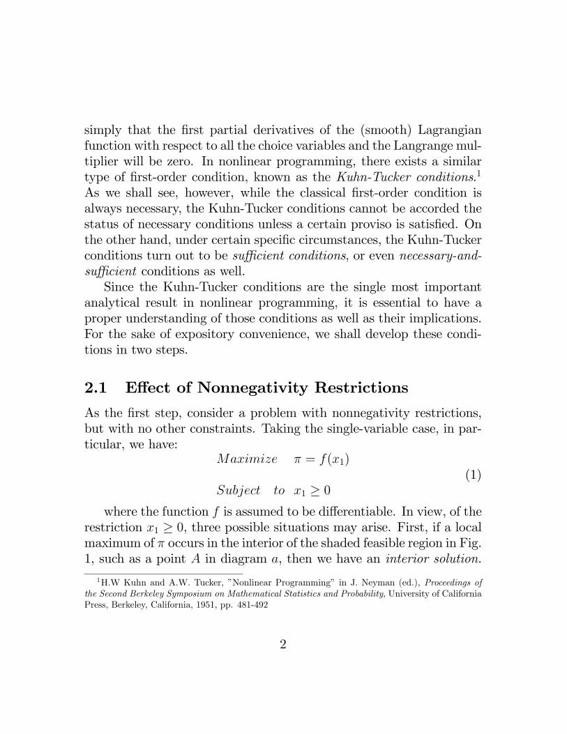
where the function f is assumed to be differentiable. In view, of therestriction x1 ≥ 0, three possible situations may arise. First, if a localmaximum of π occurs in the interior of the shaded feasible region in Fig.1, such as a point A in diagram a, then we have an interior solution.
1H.W Kuhn and A.W. Tucker, ”Nonlinear Programming” in J. Neyman (ed.), Proceedings ofthe Second Berkeley Symposium on Mathematical Statistics and Probability, University of CaliforniaPress, Berkeley, California, 1951, pp. 481-492
2
π = f(x1)
0
E
A
x1
π = f(x1)
0x1
B
π = f(x1)
0x1
C
D
(a) (b) (c)
The first-order condition in this case is dπ/dx1 = f ′(x1) = 0, same asin the classical problem. Second, as illustrated by point B in diagramb, a local maximum can also occur on the vertical axis, where x1 = 0.Even in this second case, where we have a boundary solution, the first-order condition f ′(x1) = 0 nevertheless remains valid. However, athird possibility, a local maximum may in the present context take theposition of point C or point D in diagram c, because to qualify as alocal maximum in the problem (1), the candidate point merely has tobe higher than the neighboring points within the feasible region. Inview of this last possibility, the maximum point in a problem like (1)can be characterized, not only by the equation f ′(x1) = 0, but also bythe inequality f ′(x1) < 0. Note on the other hand, that the oppositeinequality f ′(x1) > 0 can safely be ruled out, for at a point where thecurve is upward-sloping, we can never have a maximum, even if thatpoint is located on the vertical axis, such as point E in diagram a.The upshot of the above discussion is that, in order for a value of
x1 to give a local maximum of π in the problem (1), it must satisfyone of the following three conditions
f ′(x1) = 0 and x1 > 0 [point A] (2)
f ′(x1) = 0 and x1 = 0 [point B] (3)
f ′(x1) < 0 and x1 = 0 [points C and D] (4)
Actually, these three conditions can be consolidated into a single
3
statementf ′(x1) ≤ 0 x1 ≥ 0 and x1f
′(x1) = 0 (5)
The first inequality in (5) is a summary of the information regard-ing f ′(x1) enumerated in (2) through (4). The second inequality is asimilar summary for x1; in fact, it merely reiterates the nonnegativityrestriction of the problem. And, as for the third part of (5), we havean equation which expresses an important feature common to (2), (3),as well as (4), namely that, of the two quantities x1 and f ′(x1), at leastone must take a zero value, so that the product of the two must bezero. Taken together, the three parts of (5) constitute the first-ordernecessary condition for a local maximum in a problem where the choicevariable must be nonnegative. But going a step further, we can alsotake them to be necessary for a global maximum. This is because aglobal maximum must also be a local maximum and, as such, mustalso satisfy the necessary condition for a local maximum.When the problem contains n choice variables:Maximize
π = f(x1, x2, . . . , xn) (6)
Subject toxj ≥ 0 (j = 1, 2, . . . , n)
the classical first-order condition f1 = f2 = · · · = fn = 0 must besimiliarly modified. To do this, we can apply the same type of reasoningunderlying (5) to each choice variable, xj, taken by itself. Graphically,this amounts to viewing the horizontal axis in Fig. 1 as representingeach xj in turn. The required modification of the first-order conditionthen readily suggests itself:
With this background, we now proceed to the second step, and tryto include inequality constraints as well. For simplicity, let us firstdeal with a problem with three variables (n = 3) and two constaints(m = 2):Maximize
π = f(x1, x2, x3) (8)
Subject tog1(x1, x2, x3) ≤ r1
g2(x1, x2, x3) ≤ r2
andx1, x2, x3 ≥ 0
which, with the help of two dummy variables s1 and s2, can be trans-formed into the equivalent formMaximize
π = f(x1, x2, x3) (9)
Subject tog1(x1, x2, x3) + s1 = r1
g2(x1, x2, x3) + s2 = r2
andx1, x2, x3, s1, s2 ≥ 0
If the nonnegativity restrictions are absent, we may, in line withthe classical approach, form the Langrangian function :
Z∗ = f(x1, x2, x3) + λ1
[r1 − g1(x1, x2, x3)− s1
]+λ2
[r2 − g2(x1, x2, x3)− s2
] (10)
and write the first-order condition as
∂Z∗
∂x1=∂Z∗
∂x2=∂Z∗
∂x3=∂Z∗
∂s1=∂Z∗
∂s2=∂Z∗
∂λ1=∂Z∗
∂λ2= 0 (11)
5
But since the xj and si variables do have to be nonnegative, thefirst-order condition on those variables should be modified in accor-dance with (7). Consequently, we obtain the following set of conditionsinstead:
∂Z∗
∂xj≤ 0 xj ≥ 0 and xj
∂Z∗
∂xj= 0
∂Z∗
∂si≤ 0 si ≥ 0 and si
∂Z∗
∂si= 0
∂Z∗
∂λi= 0
(i = 1, 2j = 1, 2, 3
) (12)
Note that the derivatives ∂Z∗/∂λi are still to be set strictly equalto zero. (Why?)Each line (12) relates to a different type of variable. But we can
consolidate the last two lines and, in the process, eliminate the dummyvariable si from the first-order condition. Inasmuch as ∂Z∗/∂si = −λi,the second line tells us that we must have −λi ≤ 0, si ≥ 0 and −siλi =0, or equivalently,
si ≥ 0 λi ≥ 0 and siλi = 0 (13)
But the third line- a restatement of the constraints in (9)-meansthat si = ri− gi(x1, x2, x3). By substituting the latter into (13), there-fore, we can combine the second and third lines of (12) into:
ri − gi(x1, x2, x3) ≥ 0 λi ≥ 0 and λi[ri − gi(x1, x2, x3)
]= 0
This enables us to express the first-order condition (12) in an equiv-alent form without the dummy variables. Using the symbol gij to denote∂gi/∂xj, we now write
∂Z∗
∂xj= fj − (λ1g
1j + λ2g
2j ) ≤ 0 xj ≥ 0 and xj
∂Z∗
∂xj= 0
ri − gi(x1, x2, x3) ≥ 0 λi ≥ 0 and λi[ri − gi(x1, x2, x3)
]= 0(14)
6
These, then, are the Kuhn-Tucker conditions for the problem (8), or,more accurately, one version of the Kuhn-Tucker conditions, expressedin terms of the Lagrangian function Z∗ in (10)Now that we know the results, though, it is possible to obtain the
same set of conditions more directly by using a different Lagrangianfunction. Given the problem (21.10), let us ignore the nonnegativityrestrictions as well as the inequality signs in the constraints and writethe purely classical type of Lagrangian function Z:
Z = f(x1, x2, x3) + λ1
[r1 − g1(x1, x2, x3)
]+ λ2
[r2 − g2(x1, x2, x3)
](15)
Then let us (1) set the partial derivatives ∂Z/∂xj ≤ 0, but ∂Z/∂λi ≥0, (2) impose nonnegativity restrictions on xj and λi, and (3) requirecomplementary slackness to prevail between each variable and the par-tial derivative of Z with respect to that variable, that is, require theirproduct to vanish. Since the results of these steps, namely,
∂Z∂xj
= fj − (λ1g1j + λ2g
2j ) ≤ 0 xj ≥ 0 and xj
∂Z∗
∂xj= 0
∂Z∂λi
= ri − gi(x1, x2, x3) ≥ 0 λi ≥ 0 and λi∂Z∂λi
= 0(16)
are identical with (14), the Kuhn-Tucker conditions are expressiblealso in terms of the Lagrangian function Z (as against Z∗). Notethat, by switching from Z∗ to Z, we can not only arrive at the Kuhn-Tucker conditions more directly, but also identify the expression ri −gi(x1, x2, x3)-which was left nameless in (14)-as the partial derivative∂Z/∂λi. In the subsequent discussion, therefore, we shall only use the(16) version of the Kuhn-Tucker conditions, based on the Lagrangianfunction Z.
7
2.2.1 Example: UtilityMaximization with a simple rationingconstraint
Consider a familiar problem of utility maximization with a budgetconstraint:
Maximize U = U(x, y)
subject to B = PXx+ Pyy
But where a ration on x has been imposed equal to x. The Lagrangebecomes
Maxx,y
U(x, y) + λ1(B − PxX − PyY ) + λ2(x− x)
The Kuhn-Tucker conditions are
Lx = Ux − Pxλ1 − λ2 ≤ 0 x ≥ 0 and Lx · x = 0Ly = Uy − Pyλ1 ≤ 0 y ≥ 0 and Ly · y = 0Lλ1 = B − PxX − PyY ≥ 0 λ1 ≥ 0 and Lλ1 · λ1 = 0Lλ2 = x− x ≥ 0 λ2 ≥ 0 and Lλ2 · λ2 = 0
Now let us interpret the Kuhn-Tucker conditions for this particularproblem. Looking at the Lagrange
U(x, y) + λ1(B − Pxx− Pyy) + λ2(x− x)
We require thatλ1(B − Pxx− Pyy) = 0
therefore eitherλ1 = 0or
B − Pxx− Pyx = 0
8
If we interpret λ1as the marginal utility of the budget (Income),then if the budget constraint is not met the marginal utility of addi-tional B is zero (λ1 = 0).(2) Similarly for the ration constraint, either
x− x = 0or
λ2 = 0
λ2 can be interpreted as the marginal utility of relaxing the con-straint.
Numerical example
Maximize U = xy
subject to:100 ≥ x+ y
andx ≤ 40
The Lagrange is
xy + λ1(100− x− y) + λ2(40− x)
and the Kuhn-Tucker conditions become
Lx = y − λ1 − λ2 ≤ 0 x ≥ 0 and Lx · x = 0Ly = x− λ1 ≤ 0 y ≥ 0 and Ly · y = 0Lλ1 = 100− x− y ≥ 0 λ1 ≥ 0 and Lλ1 · λ1 = 0Lλ2 = 40− x ≥ 0 λ2 ≥ 0 and Lλ2 · λ2 = 0
Which gives us four equations and four unknowns: x, y, λ1 and λ2.
9
To solve, we typically approach the problem in a stepwise manner.First, ask if any λi could be zero Try λ2 = 0 (λ1 = 0 does not makesense, given the form of the utility function), then
x− λ1 = y − λ1 or x = y
from the constraint 100−x−y we get x∗ = y∗ = 50 which violates ourconstraint x ≤ 40. Therefore x∗ = 40 and y∗ = 60, also λ∗1 = 40 andλ∗2 = 20
2.3 Interpretation of the Kuhn-Tucker Conditions
Parts of the Kuhn-Tucker conditions (16) are merely a restatementof certain aspects of the given problem. Thus the conditions xj ≥ 0merely repeat the nonnegativity restrictions, and the conditions ∂Z/∂λi ≥0 merely reiterate the constraints. To include these in (16), however,has the important advantage of revealing more clearly the remarkablesymmetry between the two types of variables, xj (choice variable) andλi (Lagrange multpliers). To each variable in each category, therecorresponds a marginal condition-∂Z/∂xj ≤ 0 or ∂Z/∂λi ≥ 0-to besatisfied by the optimal solution. Each of the variables must be non-negative as well. And, finally, each variable is characterized by com-plementary slackness in relation to a particular partial derivative ofthe Lagrangian function Z. This means that, for each xj, we must findin the optimal solution that either the marginal condition holds anequality, as in the classical context, or the choice variable in questionmust take a zero value, or both. Analogously, for each λi, we mustfind in the optimal solution that either the marginal condition holdsas an equality-meaning that the i th constraint is exactly satisfied-orthe Lagrange multiplier vanishes, or both.An even more explicit interpretation is possible, when we look at
the expanded expressions for ∂Z/∂xj and ∂Z/∂λi in (16). Assume theproblem to be the familiar production problem. Then we have
10
fj ≡ the marginal gross profit of the j th productλi ≡ the shadow price of the i th resourcegij ≡ the amount of the i th resource used up in producing the
marginal unit of the j th productλig
ij ≡ the marginal imputed cost of the i th resource incurred in
producing a unit of the j th product∑i
λigij ≡ the aggregate marginal imputed cost of the j th product
Thus the marginal condition∂Z∂xj
= fj −∑i
λigij ≤ 0
requires that the marginal gross profit of the j th product be nogreater that its aggregate marginal imputed cost; i.e., no under imputationis permitted. The complementary-slackness condition then means that,if the optimal solution calls for the active production of the j th prod-uct (x∗j > 0), the marginal gross profit must be exactly equal to theaggregate marginal imputed cost (∂Z/∂x∗j = 0), as would be the situ-ation in the classical optimization problem. If, on the other hand, themarginal gross profit optimally falls short of the aggregate imputedcost (∂Z/∂x∗j < 0), entailing excess imputation, then that productmust not be produced (x∗j = 0).2 This latter situation is somethingthat can never occur in the classical context, for if the marginal grossprofit is less then the marginal imputed cost, then the output shouldin that framework be reduced all the way to the level where the mar-ginal condition is satisfied as an equality. What causes the situationof ∂Z/∂x∗j < 0 to qualify as an optimal one here, is the explicit speci-fication of nonnegativity in the present framework. For then the mostwe can do in the way of output reduction is to lower production to thelevel x∗j = 0, and if we still find ∂Z/∂x∗j < 0 at the zero output, westop there anyway.
2Remember that, given the equation ab = 0, where a and b are real numbers, we can legitimatelyinfer that a 6= 0 implies b = 0, but it is not true that a = 0 implies b 6= 0, since b = 0 is also consistentwith a = 0.
11
As for the remaining conditions, which relate to the variables λi,their meanings are even easier to percieve. First of all, the marginalcondition ∂Z/∂λi ≥ 0 merely requires the firm to stay within thecapacity limitation of every resource in the plant. The complementary-slackness condition then stipulates that, if the i th resource is notfully used in the optimal solution (∂Z/∂λ∗i > 0), the shadow price ofthat resource-which is never allowed to be negative- must be set equalto zero (λ∗i = 0). On the other hand, if a resource has a positiveshadow price in the optimal solution (λ∗i > 0), then it is perforce afully utilized resource (∂Z/∂λ∗i = 0). These, of course, are nothing butthe implications of Duality Theorem II of the preceeding chapter.It is also possible, of course, to take the Lagrange-multiplier value
λ∗i to be a measure of how the optimal value of the objective func-tion reacts to a slight relaxation of the i th constraint. In that light,complementary slackness would mean that, if the i th constraint isoptimally not minding (∂Z/∂λ∗i > 0), then relaxing that particularconstraint will not affect the optimal value of the gross profit (λ∗i = 0)-just as loosening a belt which is not constricting one’s waist to beginwith will not produce any greater comfort. If, on the other hand, aslight relaxation of the i th constraint (increasing the endowment ofthe i th resource) does increase the gross profit (λ∗i > 0), then thatresource constraint must in fact be binding in the optimal solution(∂Z/∂λ∗i = 0).
2.4 The n-Variable m-Constraint Case
The above discussion can be generalized in a straightforward manner towhen there are n choice variables and m constraints. The Lagrangian
12
function Z will appear in the more general form
Z = f(x1, x2, . . . , xn) +m∑i=1
λi[ri − gi(x1, x2, . . . , xn)
](17)
And the Kuhn-Tucker conditions will be simply be
∂Z∂xj≤ 0 xj ≥ 0 and xj
∂Z∂xj
= 0 [maximization]
∂Z∂λi≥ 0 λi ≥ 0 and λi
∂Z∂λi
= 0
(i = 1, 2, . . . ,mj = 1, 2, . . . , n
)(18)
Here, in order to avoid a cluttered appearance, we have not writtenout the expanded expressions for the partial derivatives ∂Z/∂xj and∂Z/∂λi. But you are urged to write them out for a more detailedview of the Kuhn-Tucker conditions, similar to what was given in (16).Note that, aside from the change in the dimension of the problem,the Kuhn-Tucker conditions remain entirely the same as in the three-variable, two constraint case discussed before. The interpretation ofthese conditions should naturally also remain the same.What if the problem is one of minimization? One way of handling
it is to convert the problem into a maximization problem and thenapply (6). To minimize C is equivalent to maximizing −C, so sucha conversion is always feasible. But we must, of course, also reversethe constraint inequalities by multiplying every constraint through by-1. Instead of going through the conversion process, however, we may-again using the Lagrangian function Z as defined in (17)-directly applythe minimization version of the Kuhn-Tucker conditions as follows:
∂Z∂xj≥ 0 xj ≥ 0 and xj
∂Z∂xj
= 0 [minimization]
∂Z∂λi≤ 0 λi ≥ 0 and λi
∂Z∂λi
= 0
(i = 1, 2, . . . ,mj = 1, 2, . . . , n
)(19)
13
This you should compare with (18).Reading (18) and (19) horizontally (rowwise), we see that the
Kuhn-Tucker conditions for both maximization andminimization prob-lems consist of a set of conditions relating tot he choice variables xj(first row) and another set relating to the Lagrange multipliers λi(second row). Reading them vertically (columnwise) on the otherhand, we note that, for each xj and λi, there is a marginal condi-tion (first column), a nonnegativity restriction (second column), and acomplementary-slackness condition (third column). In any given prob-lem, the marginal conditions pertaining to the choice variables alwaysdiffer, as a group, from the marginal conditions for the Lagrange mul-tipliers in the sense of inequality they take.Subject to the proviso to be explained in the next section, the
Kuhn-Tucker maximum conditions (18) and minimum conditions (19)are necessary conditions for a local maximum and local minimum, re-spectively. But since a global maximum (minimum) must also be alocal maximum (minimum), the Kuhn-Tucker conditions can also betaken as necessary conditions for a global maximum (minimum), sub-ject to the same proviso.
2.4.1 An Example
Let us check whether the Kuhn-Tucker conditions are satisfied by thesolution to the following:Minimize
Since the problem is one of minimization, the appropriate condi-tions are (19), which include the four marginal conditions
∂Z∂x1
= 2(x1 − 4)− 2λ1 + 3λ2 ≥ 0∂Z∂x2
= 2(x2 − 4)− 3λ1 + 2λ2 ≥ 0∂Z∂λ1
= 6− 2x1 − 3x2 ≤ 0∂Z∂λ2
= −12 + 3x1 + 2x2 ≤ 0
plus the nonnegativity and complementary-slackness conditions.The question is: Can we find nonnegativity values λ∗1 and λ
∗2 which,
together with the optimal values x∗1 = 2 213 = 28
13 and x∗2 = 210
13 = 3613 , will
satisfy all those conditions?Given that x∗1 and x
∗2 are both nonzero, complementary-slackness
dictates that ∂Z/∂x1 = 0 and ∂Z/∂x2 = 0, ∂Z/∂λ∗1 < 0 and ∂Z/∂λ∗2 =0, which satisfy the marginal inequalities as well as the complementary-slackness conditions, all the Kuhn-Tucker minimum conditions are sat-isfied.
2.4.2 Problems:
1. Draw a set of diagrams similar to Fig. 21.3 for the minimizationcase, and deduce a set of necessary conditions for a local mini-mum corresponding to (1.5) through (1.7). Then condense theseconditions into a single statement similar to (1.8).
(a) Show that, in (1.21), instead of writing
yi∂Z
∂λi= 0 (i = 1, . . . ,m)
15
as a set of m separate conditions, it is suffi cient to write asingle equation in the form of
m∑i=1
λi∂Z
∂λi= 0
(b) Can we do the same for the set of conditions
xj∂Z
∂xj= 0 (j = 1, . . . , n)
2. Based on the reasoning used in the preceding problem, which set(or sets) of conditions in (1.22) can be condensed into a singleequation?
3. Given the minimization problem (1.3), and using the Lagrangianfunction (1.20), take the derivatives of ∂Z/∂xj and ∂Z/∂λi andwrite out the expanded version of the Kuhn-Tucker minimumconditions (1.22).
4. Convert the minimization problem (1.3) into a maximizationproblem, formulate the Lagrangian function, take the derivativeswith respect to xj and yi, and apply the Kuhn-Tucker maximumconditions (1.21). Are the results consistent with those obtainedin the preceding problem?
5. Check the applicability of the Kuhn-Tucker conditions to Exam-ple 2 of Sec. 21.1 as follows:
(a) Write the Lagrangian function and the Kuhn-Tucker condi-tions
(b) From the solution given in Fig. 21.1b, find the optimalvalues of ∂Z/∂λi(i = 1, 2, 3). What can we conclude aboutλ∗i ?
16
(c) Now find the optimal values of ∂Z/∂x1 and ∂Z/∂x2.(d) Are all Kuhn-Tucker conditions satisfied?
3 The Constraint QualificationThe Kuhn-Tucker conditions are necessary conditions only if a par-ticular proviso is satisfied. That proviso, called the constraint quali-fication, imposes a certain restriction on the constraint functions of anonlinear program, for the specific purpose of ruling out certain irreg-ularities on the boundary of the feasible set, that would invalidate theKuhn-Tucker conditions should the optimal solution occur there.
3.1 Irregularities at Boundary Points
Let us first illustrate the nature of such irregularities by means of someconcrete examples.Example 1Maximize
π = x1
Subject tox2 − (1− x1)
3 ≤ 0
andx1, x2 ≥ 0
As shown in Fig. 2, the feasible region is the set of points thatlie in the first quadrant on or below the curve x2 = (1 − x1)
3. Sincethe objective function directs us to maximize x1, the optimal solutionis the point (1,0). But the solution fails to satisfy the Kuhn-Tuckermaximum conditions. To check this, we first write the Lagrangianfunction
Z = x1 + λ1
[−x2 + (1− x1)
3]
17
x2
0x1
x2 = (1 x1)31
1
(1,0)
As the first marginal condition, we should then have
∂Z
∂x1= 1− 3λ1(1− x1)
2 ≤ 0
In fact, since x∗1 = 1 is positive, complementary slackness requiresthat this derivative vanish when evaluated at the point (1,0). However,the actual value we get happens to be ∂Z /∂x∗1 = 1, thus violating theabove marginal condition.The reason for this anomaly is that the optimal solution (1,0), oc-
curs in this example at an outward-pointing cusp, which constitutesone type of irregularity that can invalidiate the Kuhn-Tucker condi-tions at a boundary optimal solution. A cusp is a sharp point formedwhen a curve takes a sudden reversal in direction, such that the slopeof the curve on one side of the point is the same as the slope of thecurve on the other side of the point. Here, the boundary of the feasibleregion at first follows the constraint curve, but whent the point (1,0) isreached, it takes an abrupt turn westward and follows the trail of thehorizontal axis thereafter. Since the slopes of both the curved side and
18
the horizontal side of the boundary are zero at the point (1,0), thatthe point is a cusp.Cusps are the most frequently cited culprits for the failure of the
Kuhn-Tucker conditions, but the truth is that the presence of a cuspis neither necessary nor suffi cient to cause those conditions to fail atan optimal solution. The following two examples will confirm this.
Example 2To the problem of the preceeding example, let us add a new con-
straint2x1 + x2 ≤ 2
whose border, x2 = 2 − 2x1, plots as a straight line with slope -2which passes through the optimal point in Fig. 2. Clearly, the feasibleregion remains the same as before, as so does the optimal solution atthe cusp. But if we write the new Lagrangian function
Z = x1 + λ1
[−x2 + (1− x1)
3]
+ λ2 [2− 2x1 − x2]
and the marginal conditions
∂Z∂x1
= 1− 3λ1(1− x1)2 − 2λ2 ≤ 0
∂Z∂x2
= −λ1 − λ2 ≤ 0∂Z∂λ1
= −x2 + (1− x1)3 ≥ 0
∂Z∂λ2
= 2− 2x1 − x2 ≥ 0
it turns out that the values x∗1 = 1, x∗2 = 0, λ∗1 = 1, λ∗2 = 12 do
satisfy the above four inequalities, as well as the nonnegativity andcomplementary-slackness conditions. As a mater of fact, λ∗1 can beassigned any nonnegativity value (not just 1), and all the conditionscan still be satisfied- which goes to show that the optimal value of aLagrange multiplier is not necessarily unique. More importantly, how-ever, this example shows that the Kuhn-Tucker conditions can remainvalid despite the cusp.
19
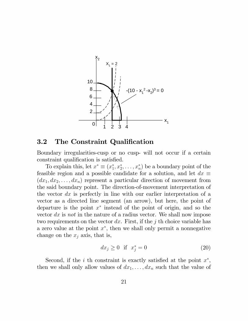
Example 3The feasible region of the problemMaximize
π = x2 − x21
Subject to−(10− x2
1 − x2)3 ≤ 0
−x1 ≤ −2
andx1, x2 ≥ 0
as shown in Fig.21.5, contains no cusp anywhere. Yet, at the op-timal solution, (2,6), the Kuhn-Tucker conditions nonetheless fail tohold. For, with the Lagrangian function
Z = x2 − x21 + λ1(10− x2
1 − x2)3 + λ2(−2 + x1)
the second marginal condition would require that
∂Z
∂x2= 1− 3λ1(10− x2
1 − x2)2 ≤ 0
Indeed, since x∗2 is positive, this derivative should vanish when eval-uated at the point (2,6). But actually we get ∂Z/∂x2 = 1, regardlessof the value assigned to λ1. Thus the Kuhn-Tucker conditions canfail even in the absence of a cusp-nay, even when the feasible regionis a convex set as in Fig. 21.5. The fundamental reason why cuspsare neither nor suffi cient for the failure of the Kuhn-Tucker conditionsis that the irregularities referred to above relate, not to the shape ofthe feasible region per se, but to the forms of the constraint functionsthemselves.
20
x2
0x1
(10 x12 x2)
3 = 0
10
2468
1 2 3 4
X1 = 2
3.2 The Constraint Qualification
Boundary irregularities-cusp or no cusp- will not occur if a certainconstraint qualification is satisfied.To explain this, let x∗ ≡ (x∗1, x
∗2, . . . , x
∗n) be a boundary point of the
feasible region and a possible candidate for a solution, and let dx ≡(dx1, dx2, . . . , dxn) represent a particular direction of movement fromthe said boundary point. The direction-of-movement interpretation ofthe vector dx is perfectly in line with our earlier interpretation of avector as a directed line segment (an arrow), but here, the point ofdeparture is the point x∗ instead of the point of origin, and so thevector dx is not in the nature of a radius vector. We shall now imposetwo requirements on the vector dx. First, if the j th choice variable hasa zero value at the point x∗, then we shall only permit a nonnegativechange on the xj axis, that is,
dxj ≥ 0 if x∗j = 0 (20)
Second, if the i th constraint is exactly satisfied at the point x∗,then we shall only allow values of dx1, . . . , dxn such that the value of
21
the constraint function gi(x∗) will not increase (for a maximization) orwill not decrease (for a minimization problem), that is,
dgi(x∗) = gi1dx1 + gi2dx2 + · · ·+ gindxn
{≤ 0 (maximization)≥ 0 (minimization)
}(21)
if gi(x∗) = ri
where all the partial derivatives of gij are to be evaluated at x∗. If
a vector dx satisfies (20) and (21), we shall refer to it as a test vector.Finally, if there exists a differentiable arc that (1) emanates from thepoint x∗, (2) is contained entirely in the feasible region, and (3) istangent to a given test vector, we shall call it a qualifying arc for thattest vector. With this background, the constraint qualification can bestated simply as follows:The constraint qualification is satisfied if, for any point x∗ on the
boundary of the feasible region, there exists a qualifying arc for everytest vector dx.
Example 4We shall show that the optimal point (1,0) of Example 1 in Fig.
2, which fails the Kuhn-Tucker conditions, also fails the constraintqualification. At that point, x∗2 = 0, thus the test vector must satisfy:
dx2 ≥ 0 [by (20)]
Moreover, since the (only) constraint, g1 = x2 − (1 − x1)3 ≤ 0, is
exactly satisfied at (1,0), we must let
g11dx1 + g1
2dx2 = 3(1− x1)2dx1 + dx2 = dx2 ≤ 0
These two requirements together imply that we must let dx2 = 0.In constrast, we are free to choose dx1. Thus, for instance, the vector
22
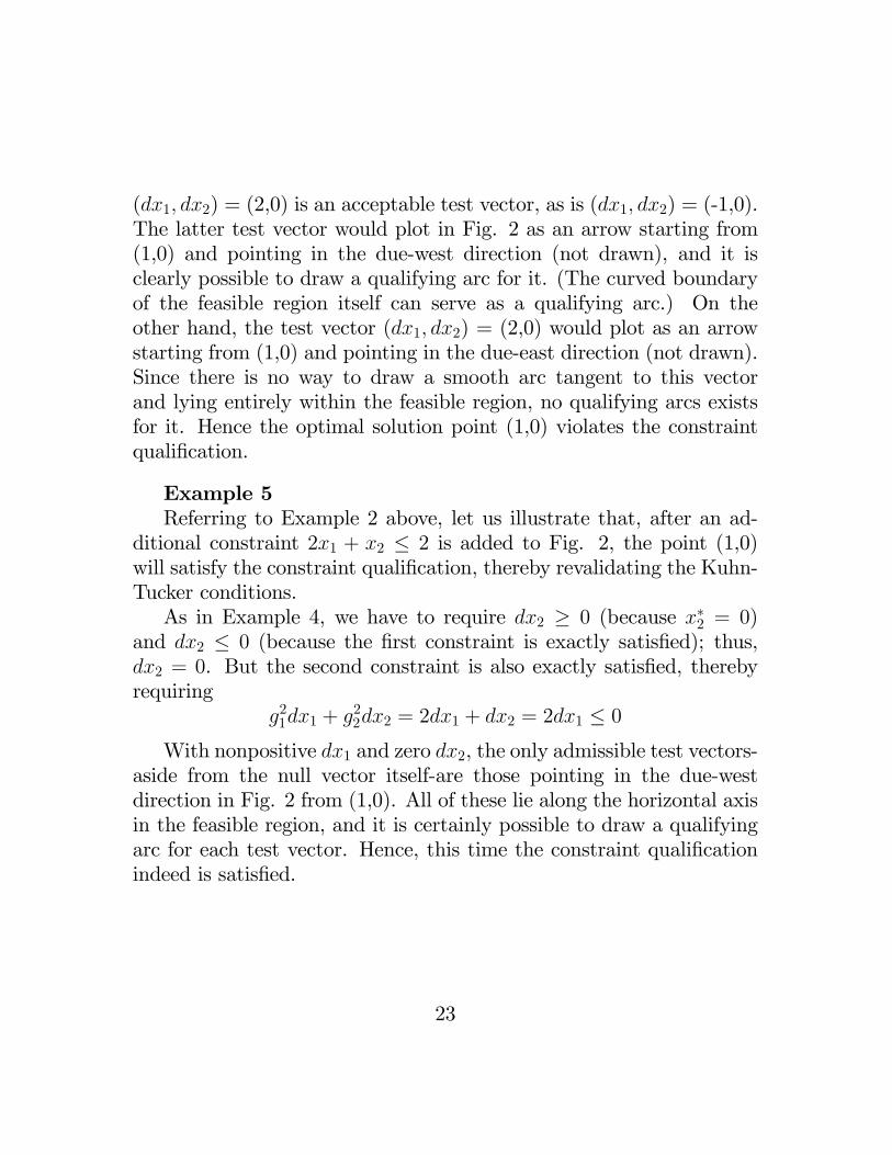
(dx1, dx2) = (2,0) is an acceptable test vector, as is (dx1, dx2) = (-1,0).The latter test vector would plot in Fig. 2 as an arrow starting from(1,0) and pointing in the due-west direction (not drawn), and it isclearly possible to draw a qualifying arc for it. (The curved boundaryof the feasible region itself can serve as a qualifying arc.) On theother hand, the test vector (dx1, dx2) = (2,0) would plot as an arrowstarting from (1,0) and pointing in the due-east direction (not drawn).Since there is no way to draw a smooth arc tangent to this vectorand lying entirely within the feasible region, no qualifying arcs existsfor it. Hence the optimal solution point (1,0) violates the constraintqualification.
Example 5Referring to Example 2 above, let us illustrate that, after an ad-
ditional constraint 2x1 + x2 ≤ 2 is added to Fig. 2, the point (1,0)will satisfy the constraint qualification, thereby revalidating the Kuhn-Tucker conditions.As in Example 4, we have to require dx2 ≥ 0 (because x∗2 = 0)
and dx2 ≤ 0 (because the first constraint is exactly satisfied); thus,dx2 = 0. But the second constraint is also exactly satisfied, therebyrequiring
g21dx1 + g2
2dx2 = 2dx1 + dx2 = 2dx1 ≤ 0
With nonpositive dx1 and zero dx2, the only admissible test vectors-aside from the null vector itself-are those pointing in the due-westdirection in Fig. 2 from (1,0). All of these lie along the horizontal axisin the feasible region, and it is certainly possible to draw a qualifyingarc for each test vector. Hence, this time the constraint qualificationindeed is satisfied.
23
x2
0x1
a11x1 + a12x2 = r1(slope = a11/a12)
a21x1 + a22x2 = r2(slope = a21/a22)
R N M
L
KJ
S
3.3 Linear Constraints
Earlier, in Example 3, it was demonstrated that te convexity of the fea-sible set does not guarantee the validity of the Kuhn-Tucker conditionsas necessary conditions. However, if the feasible region is a convex setformed by linear constraints only, then the constraint qualification willinvariably be met, and the Kuhn-Tucker conditions will always hold atan optimal solution. This being the case, we need never worry aboutboundary irregularities when dealing with a nonlinear program withlinear constraints, or, as a special case, a linear program per se.
Example 6Let us illustrate the linear-constraint result in the two-variable two-
constraint framework. For a maximization problem, the linear con-straints can be written as
a11x1 + a12x2 ≤ r1
a21x1 + a22x2 ≤ r2
where we shall take all the parameters to be positive. Then, asindicated in Fig. 21.6, the first constraint border will have a slope of
24
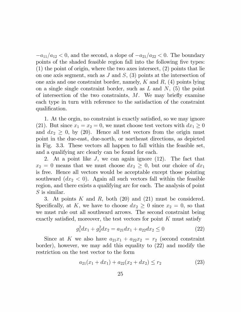
−a11/a12 < 0, and the second, a slope of −a21/a22 < 0. The boundarypoints of the shaded feasible region fall into the following five types:(1) the point of origin, where the two axes intersect, (2) points that lieon one axis segment, such as J and S, (3) points at the intersection ofone axis and one constraint border, namely, K and R, (4) points lyingon a single single constraint border, such as L and N , (5) the pointof intersection of the two constraints, M . We may briefly examineeach type in turn with reference to the satisfaction of the constraintqualification.
1. At the orgin, no constraint is exactly satisfied, so we may ignore(21). But since x1 = x2 = 0, we must choose test vectors with dx1 ≥ 0and dx2 ≥ 0, by (20). Hence all test vectors from the origin mustpoint in the due-east, due-north, or northeast directions, as depictedin Fig. 3.3. These vectors all happen to fall within the feasible set,and a qualifying arc clearly can be found for each.2. At a point like J , we can again ignore (12). The fact that
x2 = 0 means that we must choose dx2 ≥ 0, but our choice of dx1
is free. Hence all vectors would be acceptable except those pointingsouthward (dx2 < 0). Again all such vectors fall within the feasibleregion, and there exists a qualifying arc for each. The analysis of pointS is similar.3. At points K and R, both (20) and (21) must be considered.
Specifically, at K, we have to choose dx2 ≥ 0 since x2 = 0, so thatwe must rule out all southward arrows. The second constraint beingexactly satisfied, moreover, the test vectors for point K must satisfy
g21dx1 + g2
2dx2 = a21dx1 + a22dx2 ≤ 0 (22)
Since at K we also have a21x1 + a22x2 = r2 (second constraintborder), however, we may add this equality to (22) and modify therestriction on the test vector to the form
a21(x1 + dx1) + a22(x2 + dx2) ≤ r2 (23)
25
Interpreting (xj + dxj) to the new value of xj attained at the ar-rowhead of a test vector, we may construe (23) to mean that all testvectors must have their arrowheads located on or below the second con-straint border. Consequently, all these vectors must again fall withinthe feasible region, and a qualifying arc can be found for each. Theanalysis of point R is analogous.4. At points such as L and N , neither variable is zero and (20) can
be ignored. However, for point N , (21) dictates that
g11dx1 + g1
2dx2 = a11dx1 + a12dx2 ≤ 0 (24)
Since pointN satisfies a11dx1+a12dx2 = r1 (first constraint border),we may add this equality to (21.23) and write
a11(x1 + dx1) + a12(x2 + dx2) ≤ r1 (25)
This would require the test vectors to have arrowheads locatedon or below the first constraint border in Fig. 21.6. Thus we obtainessentially the same kind of result encountered in the other cases. Thisanalysis of point L is analogous.5. At point M , we may again disregard (20), but this time (21)
requires all test vectors to satisfy both (22) and (24). Since we maymodify the latter conditions to the forms in (23) and (25), all testvectors must now have their arrowheads located on or below the first aswell as the second constraint borders. The result thus again duplicatesthose of the previous cases.
In this example, it so happens that, for every type of boundarypoint considered, the test vectors all lie within the feasible region.While this locational feature makes the qualifying arcs easy to find, itis by no means a prerequisite for their exsistence. In a problem with anonlinear constraint border, in particular, the constraint border itselfmay serve as a qualifying arc for some test vector that lies outside of
26
the feasible region. An example of this can be found in one of theproblems below.
3.3.1 Problems:
1. Check whether the solution point (x∗1, x∗2) = (2, 6) in Example 3
satisfies the constraint qualification.
2. Maximize π = x1
Subject to x21 + x2
2 ≤ 1and x1, x2 ≥ 0Solve graphically and check whether the optimal-solution pointsatisfies (a) the constraint qualification and (b) the Kuhn-Tuckerconditions.
3. Minimize C = x1
Subject to x21 − x2 ≥ 0
and x1, x2 ≥ 0Solve graphically. Does the optimal solution occur at a cusp?Check whether the optimal solution satisfies (a) the constraintqualification and (b) the Kuhn-Tucker minimum conditions.
4. Minimize C = 2x1 + x2
Subject to x21 − 4x1 + x2 ≥ 0
− 2x1 − 3x2 ≥ −12and x1, x2 ≥ 0Solve graphically for the global minimum, and check whether theoptimal solution satisfies (a) the constraint qualification and (b)the Kuhn-Tucker conditions.
5. Minimize C = x1
Subject to −x2 − (1− x1)3 ≥ 0
and x1, x2 ≥ 0
27
Show that (a) the optimal solution (x1, x2) = (1,0) does not sat-isfy the Kuhn-Tucker conditions , but (b) by introducing a newmultiplier λ0 ≥ 0, and modifying the Lagrangian function (1.20)to the form
Z0 = y0f(x1, x2, . . . , xn) +m∑i=1
λ1
[ri − gi(x1, x2, . . . , xn)
]the Kuhn-Tucker conditions can be satisfied at (1,0). (Note:The Kuhn-Tucker conditions on the multipliers extend to onlyλ1, . . . λm, but not to λ0.)
4 Economic Applications
4.1 War-Time Rationing
Typically during times of war the civilian population is subject to someform of rationing of basic consumer goods. Usually, the method of ra-tioning is through the use of redeemable coupons used by the govern-ment. The government will supply each consumer with an allotmentof coupons each month. In turn, the consumer will have to redeem acertain number of coupons at the time of purchase of a rationed good.This effectively means the consumer ”pays”two ”prices”at the time ofthe purchase. He or she pays both the coupon price and the monetaryprice of the rationed good. This requires the consumer to have bothsuffi cient funds and suffi cient coupons in order to buy a unit of therationed good.Consider the case of a two-good world where both goods, x and y.
are rationed. Let the consumer’s utility function be U = U(x, y). Theconsumer has a fixed money budget of B and faces the money prices Pxand Py. Further, the consumer has an allotment of coupons, denoted
28
C, which can be used to purchase both x or y at a coupon price of cxand cy. Therefore the consumer’s maximization problem isMaximize
U = U(x, y)
Subject toB ≥ Pxx+ Pyy
andC ≥ cxx+ cyy
in addition, the non-negativity constraint x ≥ 0 and y ≥ 0.The Lagrangian for the problem is
Z = U(x, y) + λ(B − Pxx− Pyy) + λ2(C − cxx+ cyy)
where λ, λ2 are the Lagrange multiplier on the budget and couponconstraints respectively. The Kuhn-Tucker conditions are
Zx = Ux − λ1Px − λ2cx ≤ 0 x ≥ 0 x · Zx = 0Zy = Uy − λ1Py − λ2cy ≤ 0 y ≥ 0 y · Zy = 0Zλ1 = B − Pxx− Pyy ≥ 0 λ1 ≥ 0 λ1 · Zλ1 = 0Zλ2 = C − cxx− cyy ≥ 0 λ2 ≥ 0 λ2 · Zλ2 = 0
Numerical ExampleLet’s suppose the utility function is of the form U = x ·y2. Further,
let B = 100, Px = Py = 1 while C = 120 and cx = 2, cy = 1.The Lagrangian becomes
Solving the problem:Typically the solution involves a certain amount of trial and error.
We first choose one of the constraints to be non-binding and solve forthe x and y. Once found, use these values to test if the constraintchosen to be non-binding is violated. If it is, then redo the procedurechoosing another constraint to be non-binding. If violation of the non-binding constraint occurs again, then we can assume both constraintsbind and the solution is determined only by the constraints.Step one: Assume λ2 = 0, λ1 > 0By ignoring the coupon constraint, the first order conditions be-
When we check our solution against the budget constraint, we findthat the budget constraint is just met. In this case, we have the un-usual result that the budget constraint is met but is not binding dueto the particular location of the coupon constraint. The student isencouraged to carefully graph the solution, paying careful attention tothe indifference curve, to understand how this result arose.
4.2 Peak Load Pricing
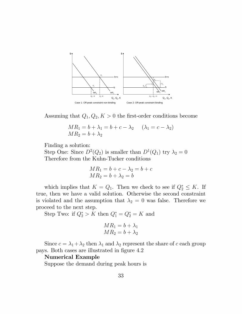
Peak and off-peak pricing and planning problems are common place forfirms with capacity constrained production processes. Usually the firmhas invested in capacity in order to target a primary market. Howeverthere may exist a secondary market in which the firm can often sellits product. Once the capital has been purchased to service the firm’sprimary market, the capital is freely available (up to capacity) to beused in the secondary market. Typical examples include: schools anduniversities who build to meet day-time needs (peak), but may offernight-school classes (off-peak); theatres who offer shows in the evening(peak) and matinees (off-peak); or trucking companies who have ded-icated routes but may choose to enter ”back-haul” markets. Sincethe capacity price is a factor in the profit maximizing decision for thepeak market and is already paid, it normally, should not be a factor incalculating optimal price and quantity for the smaller, off-peak mar-ket. However, if the secondary market’s demand is close to the samesize as the primary market, capacity constraints may be an issue, espe-cially given that it is common practice to price discriminate and chargelower prices in off-peak periods. Even though the secondary market issmaller than the primary, it is possible at the lower (profit maximizing)price that off-peak demand exceeds capacity. In such cases capacitychoices maust be made taking both markets into account, makeing theproblem a classic application of Kuhn-Tucker.Consider a profit maximizing Company who faces two demand
31
curves
P1 = D1(Q1) in the day time (peak period)P2 = D2(Q2) in the night time (off-peak period)
to operate the firm must bay b per unit of output, whether it is dayor night. Furthermore, the firm must purchase capacity at a cost of cper unit of output. Let K denote total capacity measured in units ofQ. The firm must pay for capacity, regardless if it operates in the offpeak period. Question: Who should be charged for the capacity costs?Peak, off-peak, or both sets of customers? The firm’s maximizationproblem becomes
MaximizeQ1,Q2,K
P1Q1 + P2Q2 − b(Q1 −Q2)− cK
Subject toK ≥ Q1
K ≥ Q2
WhereP1 = D1(Q1)P2 = D2(Q2)
The Lagrangian for this problem is:
Z = D1(Q1)Q1+D2(Q2)Q2−b(Q1+Q2)−cK+λ1(K−Q1)+λ2(K−Q2)
Case 1: Offpeak constraint nonbinding Case 2: Offpeak constraint binding
Assuming that Q1, Q2, K > 0 the first-order conditions become
MR1 = b+ λ1 = b+ c− λ2 (λ1 = c− λ2)MR2 = b+ λ2
Finding a solution:Step One: Since D2(Q2) is smaller than D1(Q1) try λ2 = 0Therefore from the Kuhn-Tucker conditions
MR1 = b+ c− λ2 = b+ cMR2 = b+ λ2 = b
which implies that K = Q1. Then we check to see if Q∗2 ≤ K. Iftrue, then we have a valid solution. Otherwise the second constraintis violated and the assumption that λ2 = 0 was false. Therefore weproceed to the next step.Step Two: if Q∗2 > K then Q∗1 = Q∗2 = K and
MR1 = b+ λ1
MR2 = b+ λ2
Since c = λ1 +λ2 then λ1 and λ2 represent the share of c each grouppays. Both cases are illustrated in figure 4.2Numerical ExampleSuppose the demand during peak hours is
33
P1 = 22− 10−5Q1
and during off-peak hours is
P2 = 18− 10−5Q2
To produce a unit of output per half-day requires a unit of capacitycosting 8 cents per day. The cost of a unit of capacity is the samewhether it is used at peak times only or off-peak also. In addition tothe costs of capacity, it costs 6 cents in operating costs (labour andfuel) to produce 1 unit per half day (both day and evening)If we assume that the capacity constraint is binding (λ2 = 0), then
the Kuhn-Tucker conditions (above) become
λ1 = c = 8MR︷ ︸︸ ︷
22− 2× 10⁻⁵Q1
MC︷ ︸︸ ︷= b+ c = 14
18− 2× 10⁻⁵Q2 = b = 6
Solving this system gives us
Q1 = 40000
Q2 = 60000
which violates the assumption that the second constraint is non-binding(Q2 > Q1 = K).Therefore, assuming that both constraints are binding, then Q1 =
Q2 = Q and the Kuhn-Tucker conditions become
λ1 + λ2 = 8
22− 2× 10⁻⁵Q = 6 + λ1
18− 2× 10⁻⁵Q = 6 + λ2
34
which yields the following solutions
Q = K = 50000
λ1 = 6 λ2 = 2
P1 = 17 P2 = 13
Since the capacity constraint is binding in both markets, market onepays λ1 = 6 of the capacity cost and market two pays λ2 = 2.
4.2.1 Problems
1. Suppose in the above example a unit of capacity cost only 3 centsper day.
(a) What would be the profit maximizing peak and off-peakprices and quantitites?
(b) What would be the values of the Lagrange multipliers? Whatinterpretation do you put on their values?
2. Skippy lives on an island where she produces two goods, x and y,according the the production possibility frontier 200 ≥ x2 + y2,and she consumes all the goods herself. Her utility function is
u = x · y3
Skippy also faces and environmental constraint on her total out-put of both goods. The environmental constraint is given byx+ y ≤ 20
(a) Write down the Kuhn Tucker first order conditions.
(b) Find Skippy’s optimal x and y. Identify which constaintsare binding.
35
3. An electric company is setting up a power plant in a foreigncountry and it has to plan its capacity. The peak period demandfor power is given by p1 = 400− q1 and the off-peak is given byp2 = 380 − q2. The variable cost to is 20 per unit (paid in bothmarkets) and capacity costs 10 per unit which is only paid onceand is used in both periods.
(a) write down the lagrangian and Kuhn-Tucker conditions forthis problem
(b) Find the optimal outputs and capacity for this problem.
(c) How much of the capacity is paid for by each market (i.e.what are the values of λ1 and λ2)?
(d) Now suppose capacity cost is 30 per unit (paid only once).Find quantities, capacity and how much of the capacity ispaid for by each market (i.e. λ1 and λ2)?
5 Maximum Value Functions and the En-velope Theorem3
A maximum (or minimum) value function is an objective functionwhere the choice variables have been assigned their optimal values.These optimal values of the choice variables are, in turn, functionsof the exogenous variables and parameters of the problem. Once theoptimal values of the choice variables have been substituted into theoriginal objective function, the function indirectly becomes a functionof the parameters (through the parameters’ influence on the optmal
3This section of the chapter presents an overview of the envelope theorem for the purpose ofintroducing the concept to the student. For a richer treatment of this topic is found in chapter 7 ofThe Structure of Economics: a Mathematical Analysis (3rd Ed.) by Eugene Silberberg and WingSuen (McGraw-Hill, 2001) from which parts of this section are based.
36
values of the choice variables). Thus the maximum value function isalso referred to as the indirect objective function.What is the significance of the indirect objective function? Con-
sider that in any optimization problem the direct objective function ismaximized (or minimized) for a given set of parameters. The indirectobjective function gives all the maximum values of the objective func-tion as these prameters vary. Hence the indirect objective function isan ”envelope”of the set of optimized objective functions generated byvarying the parameters of the model. For most students of economicsthe first illustration of this notion of an ”envelope”arises in the com-parison of short-run and long-run cost curves. Students are typicallytaught that the long-run average cost curve is an envelope of all theshort-run average cost curves (what parameter is varying along theenvelope in this case?). A formal derivation of this concept is one ofthe exercises we will be considering in the following sections.To illustrate, consider the following maximization problem with two
choice variables x and y, and one parameter, α:Maximize
U = f(x, y, α) (26)
The first order necessary condition are
fx(x, y, α) = fy(x, y, α) = 0 (27)
if second-order conditions are met, these two equations implicitly definethe solutions
x = x∗(α) y = x∗(α) (28)
If we subtitute these solutions into the objective function, we obtain anew function
V (α) = f(x∗(α), y∗(α), α) (29)
where this function is the value of f when the values of x and yare those that maximize f(x, y, α). Therefore, V (α) is the maximum
37
value function (or indirect objective function). If we differentiate Vwith respect to α
∂V
∂α= fx
∂x∗
∂α+ fy
∂y∗
∂α+ fα (30)
However, from the first order conditions we know fx = fy = 0.Therefore, the first two terms disappear and the result becomes
∂V
∂α= fα (31)
This result says that, at the optimum, as α varies, with x∗ and y∗
allowed to adjust optimally gives the same result as if x∗ and y∗ wereheld constant! Note that α enters maximum value function (equation29) in three places: one direct and two indirect (through x∗ and y∗).Equations 30 and 31 show that, at the optimimum, only the directeffect of α on the objective function matters. This is the essence of theenvelope theorem. The envelope theorem says only the direct effects ofa change in an exogenous variable need be considered, even though theexogenous variable may enter the maximum value function indirectlyas part of the solution to the endogenous choice variables.
5.1 The Profit Function
Let’s apply the above approach to an economic application, namelythe profit function of a competitive firm. Consider the case where afirm uses two inputs: capital, K, and labour, L. The profit function is
π = pf(K,L)− wL− rK (32)
where p is the output price and w and r are the wage rate andrental rate respectively.
38
The first order conditions are
πL = fL(K,L)− w = 0πK = fK(K,L)− r = 0
(33)
which respectively define the factor demand equations
L = L∗(w, r, p)K = K∗(w, r, p)
(34)
substituting the solutions K∗ and L∗ into the objective functiongives us
π∗(w, r, p) = pf(K∗, L∗)− wL∗ − rK∗ (35)
π∗(w, r, p) is the profit function (or indirect objective function).The profit function gives the maximum profit as a function of theexogenous variables w, r, and p.Now consider the effect of a change in w on the firm’s profits. If we
differentiate the original profit function (equation 32) with respect tow, holding all other variables constant and we get
∂π
∂w= −L (36)
However, this result does not take into account the profit maximiz-ing firms ability to make a substitution of capital for labour and adjustthe level of output in accordance with profit maximizing behavior.Since π∗(w, r, p) is the maximum value of profits for any values of w,
r, and p, changes in π∗ from a change in w takes all captial for laboursubsitutions into account. To evaluate a change in the maximum profitfunction from a change in w, we differentiate π∗(w, r, p) with respectto w yielding
∂π∗
∂w= [pfL − w]
∂L∗
∂w+ [pfK − r]
∂K∗
∂w− L∗ (37)
39
From the first order conditions, the two bracketed terms are equalto zero. Therefore, the resulting equation becomes
∂π∗
∂w= −L∗(w, r, p) (38)
This result says that, at the the profit maximizing position, achange in profits with respect to a change in the wage is the samewhether or not the factors are held constant or allowed to vary as thefactor price changes. In this case the derivative of the profit func-tion with respect to w is the negative of the factor demand functionL∗(w, r, p). Following the above procedure, we can also show the ad-ditional comparative statics results
∂π∗(w, r, p)
∂r= −K∗(r, w, p) (39)
and∂π∗(w, r, p)
∂p= f(K∗, L∗) = q∗ (40)
The simple comparative static results derived from the profit func-tion is known as ”Hotelling’s Lemma”. Hotelling’s Lemma is simplyan application of the envelope theorem.
5.2 Reciprocity Conditions
Consider again our two variable maximization problem
Maximize U = f(x, y, α)
where x and y are the choice variable, and α is a parameter. The firstorder equations are fx = fy = 0. which imply the functions x = x∗(α)and y = y∗(α).
40
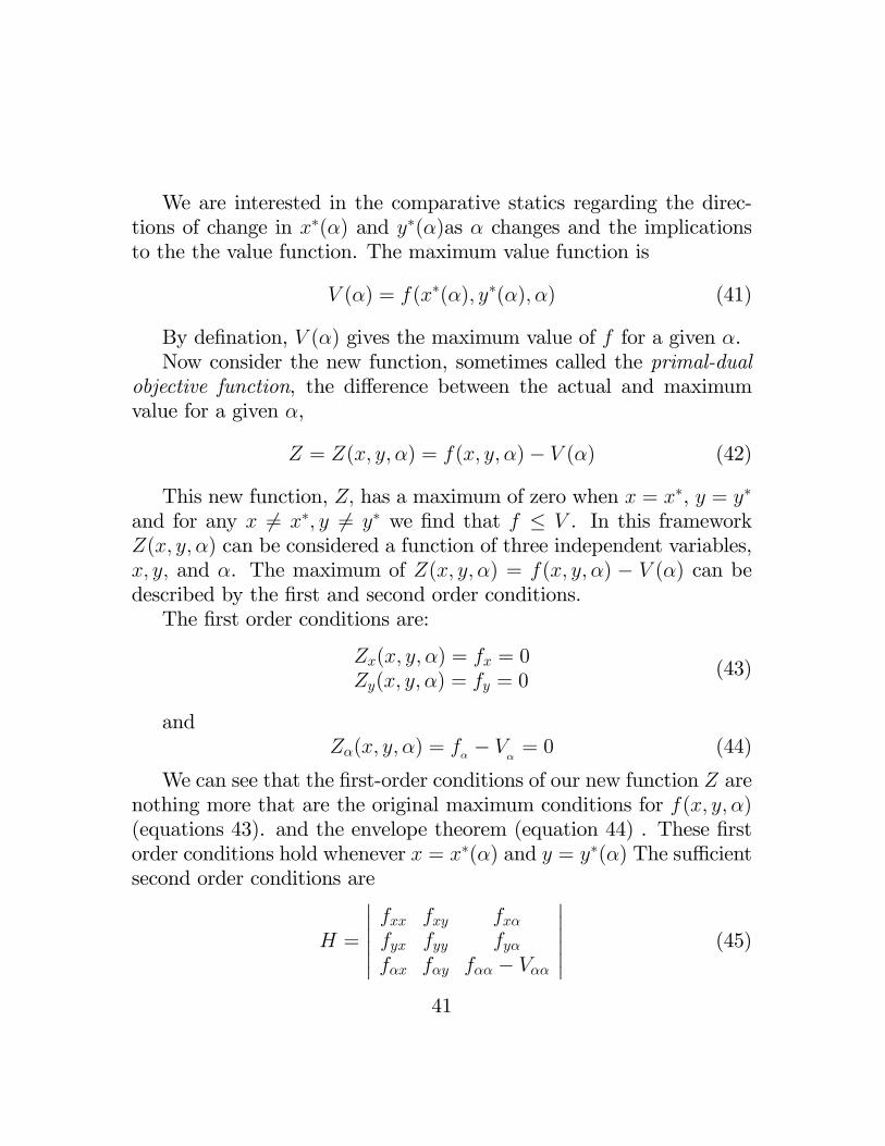
We are interested in the comparative statics regarding the direc-tions of change in x∗(α) and y∗(α)as α changes and the implicationsto the the value function. The maximum value function is
V (α) = f(x∗(α), y∗(α), α) (41)
By defination, V (α) gives the maximum value of f for a given α.Now consider the new function, sometimes called the primal-dual
objective function, the difference between the actual and maximumvalue for a given α,
Z = Z(x, y, α) = f(x, y, α)− V (α) (42)
This new function, Z, has a maximum of zero when x = x∗, y = y∗
and for any x 6= x∗, y 6= y∗ we find that f ≤ V . In this frameworkZ(x, y, α) can be considered a function of three independent variables,x, y, and α. The maximum of Z(x, y, α) = f(x, y, α) − V (α) can bedescribed by the first and second order conditions.The first order conditions are:
Zx(x, y, α) = fx = 0Zy(x, y, α) = fy = 0
(43)
andZα(x, y, α) = f
α− V
α= 0 (44)
We can see that the first-order conditions of our new function Z arenothing more that are the original maximum conditions for f(x, y, α)(equations 43). and the envelope theorem (equation 44) . These firstorder conditions hold whenever x = x∗(α) and y = y∗(α) The suffi cientsecond order conditions are
H =
∣∣∣∣∣∣fxx fxy fxαfyx fyy fyαfαx fαy fαα − Vαα
∣∣∣∣∣∣ (45)
41
where the Hessian Matrix is negative definite, or
fxx < 0, fxxfyy − f 2xy > 0, H < 0 (46)
In addition, if the the second-order conditions are met, then fαα −Vαα < 0 is also implied. This inequality is an important result whichplays an essential role in many comparitive static exercises. We knowalready that
Vα(α) = fα(x∗(α), y∗(α), α) (47)
Differentiating both sides with respect to α yields
Vαα = fαx∂x∗
∂α− fαy
∂y∗
∂α+ fαα (48)
From the suffi cient second order conditions and using Young’s the-orem
Vαα − fαα = fxα∂x∗
∂α+ fyα
∂y∗
∂α> 0 (49)
Suppose that α enters only in the x first order condition such thatfyα = 0 Then equation 49 reduces to
fxα∂x∗
∂α> 0 (50)
which implies that fxα and ∂x∗
∂α will have the same sign4.
For example, in the profit maximization model:
π = pf(K,L)− wL− rK (51)
Where the first order conditions are
πL = pfL − w = 0πK = pfK − r = 0
(52)
4This analysis is easily generalized to the n-variable case.
42
The exogenous variable w enters only the first order equation pfL−w = 0; it enters with a negative sign
∂πL∂w
= −1 (53)
Therefore we can conclude that ∂L∗/∂w will also be negative. Fur-ther, if we combine of the envelope theoremwith with Young’s theorem,we can show the reciprocity condition ∂L∗
∂r = ∂K∗
∂w . From the indirectprofit function π∗(w, r, p) Hotelling’s Lemma gave us
π∗w = ∂π∗∂w = −L∗(w, r, p)
π∗r = ∂π∗∂r = −K∗(w, r, p) (54)
differentiating again and applying Young’theorem
π∗wr = −∂L∗
∂r= −∂K
∗
∂w= π∗rw (55)
or∂L∗
∂r=∂K∗
∂w(56)
5.3 The Envelope Theorem and Constrained Op-timization
Now let us turn our attention to the case of constrained optimization.Again we will have an objective function (U), two choice variables, (xand y) and one prarameter (α) except now we introduce the followingconstraint:
g(x, y;α) = 0
The derivation of the envelope theorem for the models with oneconstraint is as follows:
Substituting the solutions into the objective function, we get
U ∗ = f(x∗(α), y∗(α), α) = V (α) (62)
where V (α) is the indirect objective function, or maximum valuefunction. This is the maximum value of y for any α and xi’s thatsatisfy the constraint.
How does V (α) change as α changes? First, we differentiate V withrespect to α
∂V
∂α= fx
∂x∗
∂α+ fy
∂y∗
∂α+ fα (63)
In this case,equation 63 will not simplify to ∂V∂α = fα since fx 6= 0
and fy 6= 0. However, if we substitute the solutions to x and y into theconstraint (producing an identity)
g(x∗(α), y∗(α), α) ≡ 0 (64)
44
and differentiating with respect to α yields
gx∂x∗
∂α+ gx
∂x∗
∂α+ gα ≡ 0 (65)
If we multiply equation 65 by λ and combine the result with equa-tion 63 and rearranging terms, we get
∂V
∂α= (fx + λgx)
∂x∗
∂α+ (fy + λgy)
∂y∗
∂α+ fα + λgα = Zα (66)
Where Zα is the partial deviative of the Lagrangian function withrespect to α, holding all other variable constant. In this case, theLangrangian functions serves as the objective function in deriving theindirect objective function.While the results in equation 66 nicely parallel the unconstrained
case, it is important to note that some of the comparative static resultsdepend critically on whether the parameters enter only the objectivefunction or whether they enter only the constraints, or enter both. If aparameter enters only in the objective function then the comparativestatic results are the same as for unconstrained case. However, if theparameter enters the constraint, the relation
Vαα ≥ fαα
will no longer hold.
5.4 Interpretation of the Lagrange Multiplier
In the consumer choice problem in chapter 12 we derived the resultthat the Lagrange multiplier, λ, represented the change in the valueof the Lagrange function when the consumer’s budget changed. Weloosely interpreted λ as the marginal utility of income. Now let us
45
derive a more general interpretation of the Lagrange multiplier withthe assistance of the envelope theorem.Consider the problemMaximize
U = f(x, y) (67)
Subject toc− g(x, y) = 0 (68)
where c is a constant. The Lagrangian for this problem is
which gives us the condition that the slope of the level curve of theobjective function must equal the slope of the constraint at the opti-mum.Equations (70) implicitly define the solutions
x = x∗(c) y = y(c) λ = λ∗(c) (72)
substituting (72) back into the Lagrangian yields the mamximumvalue function
V (c) = Z∗(c) = f (x∗(c), y∗(c)) + λ∗(c) (c− g(x∗1(c), y∗(c))) (73)
46
differentiating with respect to c yields
∂Z∗
∂c= fx
∂x∗
∂c+fy
∂y∗
∂c+(c− g(x∗(c), y∗(c)))
∂λ∗
∂c−λ∗(c)gx
∂x∗
∂c−λ∗(c)gy
∂y∗
∂c+λ∗(c)
∂c
∂c(74)
by rearranging we get
∂Z∗
∂c= (fx−λ∗gx)
∂x∗
∂c+ (fy−λ∗gy)
∂y∗
∂c+ (c−g(x∗, y∗))
∂λ∗
∂c+λ∗ (75)
Note that the three terms in brackets are nothing more than thefirst order equations and, at the optimal values of x, y and λ, theseterms are all equal to zero. Therefore this expression simplifies to
∂V (c)
∂c=∂Z∗
∂c= λ∗ (76)
Therefore equals the rate of change of the maximum value of theobjective function when c changes (λ is sometimes referred to as the”shadow price”of c).Note that, in this case, c enters the problem onlythrough the constraint; it is not an argument of the original objectivefunction.
6 Duality and the Envelope TheoremA consumer’s expenditure function and his indirect utility functionare the minimum and maximum value functions for dual problems.An expenditure function specifies the minimum expenditure requiredto obtain a fixed level of utility given the utility function and theprices of consumption goods. An indirect utility function specifies themaximum utility that can be obtained given prices, income and theutility function.
47
Let U(x, y) be a utility function in x and y are consumption goods.The consumer has a budget, B, and faces market prices Px and Py forgoods x and y respectively.Setting up the Lagrangian:
This system of equations implicitly define the solutions to xh, yh
and λhxh = xh(U ∗, Px, Py)yh = yh(U ∗, Px, Py)
λh = λh(U ∗, Px, Py)(83)
xh and yh are the compensated, or ”real income”held constant de-mand functions. They are commonly referred to as ”Hicksion”demandfunctions, hence the h superscript.6
If we compare the first two equations from the first order conditionsin both utility maximization problem and expenditure minimizationproblem (Zx, Zy), we see that both sets can be combined (eliminatingλ) to give us
Px
Py=Ux
Uy(= MRS) (84)
This is the tangency condition in which the consumer chooses theoptimal bundle where the slope of the indifference curve equals theslope of the budget constraint. The tangency condition is identicalfor both problems. If the target level of utility in the minimizationproblem is set equal to the value of the utility obtained in the solutionto the maximization problem, namely U ∗, we obtain the following
or the solution to both the maximization problelm and the mini-mization problem produce identical values for x and y. However, the
6Yet another famous, but dead economist, Sir John Hicks.
49
solutions are functions of different exogenous variables so any compar-ative statics exercises will produce different results.Substituting xh and yh into the objective function of the minimiza-
tion problem yields
Pxxh(Px, Py, U
∗) + Pyyh(Px, Py, U
∗) = E(Px, Py, U∗) (86)
where E is the minimum value function or expenditure function.The duality relationship in this case is
E(Px, Py, U∗, α) = B (87)
where B is the exogenous budget from the maximization problem.Finally, it can be shown from the first order conditions of the two
problems that
λM =1
λh(88)
6.1 Roy’s Identity
One application of the envelope theorem is the derivation of Roy’sidentity. Roy’s identity states that the individual consumer’s marshal-lian demand function is equal to the ratio of partial derviatives of themaximum value function. Substituting the optimal values of xM , yM
Next, differentiate the value function with respect to B
∂V
∂B= (Ux−λMPx)
∂xM
∂B+(Uy−λMPy)
∂yM
∂B+B−PxxM−PyyM)
∂λM
∂B+λM
(92)
∂V
∂B= (0)
∂xM
∂B+ (0)
∂yM
∂B+ (0)
∂λM
∂B+ λM = λM (93)
Finally, taking the ratio of the two partial derivatives∂V∂Px∂V∂B
=−λMxM
λM= xM (94)
which is Roy’s identity.
6.2 Shephard’s Lemma
Earlier in the chapter an application of the envelope theorem was thederivation of Hotelling’s Lemma, which states that the partial deriva-tives of the maximum value of the profit function yields the firm’s fac-tory demand functions and the supply functions. A similar approachapplied to the expenditure function yields Shepard’s Lemma.Consider the consumer’s minimization problem. The Lagrangian is
Z = Pxx+ Pyy + λ(U ∗ − U(x, y)) (95)
From the first order conditions, the solutions are implicitly defined
xh = xh(Px, Py, U∗)
yh = yh(Px, Py, U∗)
λh = λh(Px, Py, U∗)
(96)
51
Substituting these solutions into the Lagrangian yields the mini-mum value function
V (Px, Py, U∗) = Pxx
h + Pyyh + λh(U ∗ − U(xh, yh)) (97)
The partial derivatives of the value function with respect to Px andPy are the consumer’s conditional, or Hicksian, demands:
∂V∂Px
= (Px − λhUx)∂xh
∂Px+ (Py − λhUy) ∂y
h
∂Px+ (U ∗ − U(xh, yh))∂λ
h
∂Px+ xh
∂V∂Px
= (0)∂xh
∂Px+ (0) ∂y
h
∂Px+ (0)∂λ
h
∂Px+ xh = xh
(98)and
∂V∂Py
= (Px − λhUx)∂xh
∂Py+ (Py − λhUy)∂y
h
∂Py+ (U ∗ − U(xh, yh))∂λ
h
∂Py+ yh
∂V∂Py
= (0)∂xh
∂Py+ (0) ∂y
h
∂Py+ (0)∂λ
h
∂Py+ yh = yh
(99)Differentiating V with respect to the constraint U∗ yields λh, the
marginal cost of the constraint
∂V
∂U ∗= (Px − λhUx)
∂xh
∂U ∗+ (Py − λhUy)
∂yh
∂Py+ (U ∗ − U(xh, yh))
∂λh
∂U ∗+ λh
∂V
∂U ∗= (0)
∂xh
∂U ∗+ (0)
∂yh
∂U ∗+ (0)
∂λh
∂U ∗+ yh = λh
Together, these three partial derivatives are Shepard’s Lemma.
6.3 Example of duality for the consumer choiceproblem
6.3.1 Utility Maximization
Consider a consumer with the utility function U = xy, who faces abudget constraint of B = PxxPyy, where all variables are defined asbefore.
52
The choice problem isMaximize
U = xy (100)
Subject toB = PxxPyy (101)
The Lagrangian for this problem is
Z = xy + λ(B − PxxPyy) (102)
The first order conditions are
Zx = y − λPx = 0Zy = x− λPy = 0Zλ = B − Pxx− Pyy = 0
(103)
Solving the first order conditions yield the following solutions
xM = B2Px
yM = B2Py
λ = B2PxPy
(104)
where xM and yM are the consumer’s Marshallian demand func-tions. Checking second order conditions, the bordered Hessian is
∣∣H∣∣ =
∣∣∣∣∣∣0 1 −Px1 0 −Py−Px −Py 0
∣∣∣∣∣∣ = 2PxPy > 0 (105)
Therefore the solution does represent a maximum . SubstitutingxM and yM into the utility function yields the indirect utility function
V (Px, Py, B) =
(B
2Px
)(B
2Py
)=
B2
4PxPy(106)
If we denote the maximum utility by U0 and re-arrange the indirectutility function to isolate B
B2
4PxPy= U0 (107)
53
B = (4PxPyU0)12 = 2P
12
x P12
y U12
0 = E(Px, Py, U0) (108)
We have the expenditure function
Roy’s Identity Let’s verify Roy’s identity which states
xM = −∂V∂Px∂V∂B
(109)
Taking the partial derivative of V
∂V
∂Px= − B2
4P 2xPy
(110)
and∂V
∂B= − B
PxPy(111)
Taking the negative of the ratio of these two partials
−∂V∂Px∂V∂B
= −
(B2
4P 2xPy
)(
BPxPy
) =B
2Px= xM (112)
Thus we find that Roy’s Identity does hold.
6.3.2 The dual and Shepard’s Lemma
Now consider the dual problem of cost minimization given a fixed levelof utility. Letting U0 denote the target level of utility, the problem isMinimize
Pxx+ Pyy (113)
54
Subject toU0 = xy (114)
The Lagrangian for the problem is
Z = Pxx+ Pyy + λ(U0 − xy) (115)
The first order conditions are
Zx = Px − λy = 0Zy = Py − λx = 0Zλ = U0 − xy = 0
(116)
Solving the system of equations for x, y and λ
xh =(PyU0Px
) 12
yh =(PxU0Py
) 12
λh =(PxPyU0
) 12
(117)
where xh and yh are the consumer’s compensated (Hicksian) de-mand functions. Checking the second order conditions for a minimum
∣∣H∣∣ =
∣∣∣∣∣∣0 −λ −y−λ 0 −x−y −x 0
∣∣∣∣∣∣ = −2xyλ < 0 (118)
Thus the suffi cient conditions for a minimum are satisfied.Substituting xh and yh into the orginal objective function gives us
the minimum value function, or expenditure function
Pxxh + Pyy
h = Px
(PyU0Px
) 12
+ Py
(PxU0Py
) 12
= (PxPyU0)12 + (PxPyU0)
12
= 2P12
x P12y U
120
(119)
55
Note that the expenditure function derived here is identical tothe expenditure function obtained by re-arranging the indirect utilityfunction from the maximization problem.
Shepard’s Lemma We can now test Shepard’s Lemma by differen-tiating the expenditure function directly.First, we derive the conditional demand functions
∂E(Px, Py, U0)
∂Px=
∂
∂Px
(2P
12
x P12y U
120
)=P
12y U
120
P12
x
= xh (120)
and
∂E(Px, Py, U0)
∂Py=
∂
∂Py
(2P
12
x P12y U
120
)=P
12y U
120
P12
y
= yh (121)
Next, we can find the marginal cost of utility (the Lagrange multi-plier)
∂E(Px, Py, U0)
∂U 0=
∂
∂U 0
(2P
12
x P12y U
120
)=P
12x P
12y
U12
0
= λh (122)
Thus, Shepard’s Lemma holds in this example.
7 Income and Substitution Effects: TheSlutsky Equation
7.1 The Traditional Approach
Consider a representative consumer who chooses only two goods: xand y. The price of both goods are determined in the market and
56
are therefore exogenous. As well, the consumer’s budget is also exoge-nously determined. The consumer choice problem then isMaximize
U(x, y) (123)
Subject toB = PxX + PyY (124)
The Langrangian function for this optimization problem is
Z = U(x, y) + λ(B − Pxx+ Pyy) (125)
The first order conditions yield the following set of simultaneousequations:
Zλ = B − Pxx− Pyy = 0Zx = Ux − λPx = 0Zy = Uy − λPy = 0
(126)
Solving this system will allow us to express the optimal values of theendogenous variables as implicit functions of the exogenous variables:
By taking the total differential of each identity in turn, and notingthat Uxy = Uyx (Young’s Theorem), we then arrive at the linear system
−Pxdx∗ − Pydy = x∗dPx+ y∗dPy − dB−Pxdλ∗ + Uxxdx
∗ + Uxydy∗ = λ∗dPx
−Pydλ∗ + Uyxdx∗ + Uyydy
∗ = λ∗dPy(128)
Writing these equations in matrix form 0 −Px −Py−Px Uxx Uxy−Py Uyx Uyy
dλ∗
dx∗
dy∗
=
x∗dPx + y∗dPy − dBλ∗dPxλ∗dPy
To study the effect of a change in the budget, let the other exoge-
nous differentials equal zero (dPx = dPy = 0, dB 6= 0). Then dividingthrough by dB, and applying the implicit function theorem, we have 0 −Px −Py
−Px Uxx Uxy−Py Uyx Uyy
dλ∗/∂Bdx∗/∂Bdy∗/∂B
=
−100
(129)
The coeffi cient matrix of this system is the Jacobian matrix, whichhas the same value as the bordered Hessian
∣∣H∣∣ which is positive if thesecond order conditions are met. By using Cramer’s rule we can solvefor the following comparative static
∂x∗
∂B=
1∣∣H∣∣∣∣∣∣∣∣
0 −1 −Py−Px 0 Uxy−Py 0 Uyy
∣∣∣∣∣∣ =1∣∣H∣∣∣∣∣∣ −Px Uxy−Py Uyy
∣∣∣∣ =
∣∣H̄12
∣∣∣∣H∣∣ ≶ 0 (130)
58
As before, in the absence of additional information about the rel-ative magnitudes of Px, Py and the cross partials, Uij, we are un-able to ascertain the sign of this comparative-static derivative. Thismeans that the optimal x∗ may increase in the budget, B, dependingon whether it is a normal or inferior good (ambiguous income effect)Next, we may analyze the effect of a change in Px. Letting dPy =
dB = 0 but keeping dPx 6= 0 and dividing Equation 128 by dPx weobtain 0 −Px −Py
−Px Uxx Uxy−Py Uyx Uyy
∂λ∗/∂Px∂x∗/∂Px∂y∗/∂Px
=
x∗
λ∗
0
(131)
From this, the following comparative static emerges:
∂x∗
∂Px= 1
|H|
∣∣∣∣∣∣0 x∗ −Py−Px λ∗ Uxy−Py 0 Uyy
∣∣∣∣∣∣= −x∗|H|
∣∣∣∣ −Px Uxy−Py Uyy
∣∣∣∣+ λ∗
|H|
∣∣∣∣ 0 −Py−Py Uyy
∣∣∣∣= (−x∗)|H̄12|
|H| + λ∗|H̄22||H|
(132)
Note that there are two componants in ( ∂x∗
∂Px). By comparing the
first term to our previous comparative static (∂x∗
∂B ), we see that
(−x∗)∣∣H̄12
∣∣∣∣H∣∣ = (−x∗)(∂x∗
∂B
)≶ 0 (133)
which can be interpreted as the income effect of a price change.The second term is the income compensated version of ∂x∗/∂Px , or thesubstitution effect of a price change, which is unambiguously negative:(
∂x∗
∂Px
)compensated
=λ∗∣∣H∣∣∣∣∣∣ 0 −Py−Py Uyy
∣∣∣∣ = λ∗∣∣H̄22
∣∣∣∣H∣∣ =λ∗∣∣H∣∣(P 2
y ) < 0
(134)
59
Hence, we can express Equation 132 in the form
∂x∗
∂P ∗= −
(∂x∗
∂B
)x∗︸ ︷︷ ︸
Income Effect
+
(∂x∗
∂Px
)compensated︸ ︷︷ ︸
Substitution Effect
(135)
This result, which decomposes the comparative static derivative(∂x∗/∂Px) into two componants, an income effect and a substitutioneffect, is the two-good version of the ”Slutsky Equation.”
7.2 Duality and the Alternative Slutsky
From the envelope theorem, we can derive the Slutsky decomposition ina more succinct manner. Consider first that from the utility maximumproblem we derived solutions for x and y
xM = xM(Px, Py, B)yM = yM(Px, Py, B)
(136)
which were the marshallian demand functions. Substituting these so-lutions into the utility function yielded the indirect utility function (ormaximum value function)
U ∗ = U(xM(Px, Py, B), yM(Px, Py, B)) = U ∗(Px, Py, B) (137)
which could be rewritten to isolate B and giving us the expenditurefunction
B∗ = B(Px, Py,U∗) (138)
Second, from the budget minimization problem we derived theHicksian, or compensated, demand function
x∗ = xh(Px, Py,U∗) (139)
60
which, by Shephards lemma, is equivalent to the partial derivative ofthe expenditure function with respect to Px:
∂B(Px, Py,U∗)
∂Px= xc(Px, Py,U
∗) (140)
Thus we know that if the maximum value of utility obtained from
Max U(x, y) + λ(B − Pxx− Pyy)
is the same value as the exogenous level of utility found in the con-strained minimization problem
Min Pxx+ Pyy + λ(U0 − U(x, y)) (141)
the values of x and y that satisfy the first order conditions of bothproblems will be identical, or
xc(Px, Py,U0) = xm(Px, Py,B) (142)
at the optimum.If we subsitiute the expenditure function into xM
in place of the budget, B, we get
xc(Px, Py,U0) = xM(Px, Py,B∗(Px, Py,U0)) (143)
Differentiate both sides of equation 143 with respect to Px
∂xc(Px,Py,U0)∂Px
=∂xM (Px,Py,B
∗(Px,Py,U0))∂Px
+∂xM (Px,Py,B
∗(Px,Py,U0))∂B
∂B(Px,Py,U0)∂Px
(144)
But we know from Shephard’s lemma that
∂B(Px, Py,U0)
∂Px= xc (145)
61
substituting equation 145 in to equation 144 we get
∂xc
∂Px=∂xM
∂Px+ xc
∂xM
∂B(146)
Subtract (xc ∂xM
∂B ) from both sides gives us
∂xM
∂Px= −xc∂x
M
∂B︸ ︷︷ ︸Income effect
+∂xc
∂Px︸︷︷︸Substitution effect
(147)
If we compare equation (147) to equation (135) we see that we havearrived at the identical result. The method of deriving the slutskydecomposition through the application of duality and the envelopetheorem is sometimes referred to as the ”instant slutsky”.
7.2.1 Problems:
1. A consumer has the following utility function: U(x, y) = x(y+1),where x and y are quantities of two consumption goods whoseprices are px and py respectively. The consumer also has a budgetof B. Therefore the consumer’s maximization problem is
x(y + 1) + λ(B − pxx− pyy)
(a) From the first order conditions find expressions for the de-mand functions. What kind of good is y? In particularwhat happens when py > B/2?
(b) Verify that this is a maximum by checking the second or-der conditions. By substituting x∗ and y∗ into the utilityfunction find an expressions for the indirect utility function
U ∗ = U(px, py, B)
62
and derive an expression for the expenditure function
B∗ = B(px, py, U∗)
(c) This problem could be recast as the following dual problem
Minimize pxx+ pyy subject to U ∗ = x(y + 1)
Find the values of x and y that solve this minimizationproblem and show that the values of x and y are equal tothe partial derivatives of the expenditure function, ∂B/∂pxand ∂B/∂py respectively.